Lab 4
Let’s start by importing the data for edges, node attributes, and the shapefile of the area of study.
colpal <- RColorBrewer::brewer.pal(4, "Dark2")

library(dplyr)
library(sf)
library(tidygraph)
# Load data of movements and nodes
net <- STNet::SwineMov
node_attrib <- STNet::SwinePrem %>%
  mutate(idch = as.character(id)) # Format id as character to use it later
# Load the spatial object
IO <- st_read(system.file("data/Io.shp", package = "STNet"), quiet = T)
1 Introduction to dynamic networks
The networkDynamic package has functions that allow to
analyze and visualize a network and incorporate temporality to it. To
incorporate a temporal window, we need to specify the start time (onset)
and end time (termini). For the purposes of this example we will assume
that the contact time is one week.
# Load libraries
## For dynamic networks
library(networkDynamic)
# To visualize and get network statistics
library(ndtv)
library(tsna)

net <- net %>%
  mutate(date = as.Date(date, format = '%m/%d/%y'), # Format the variable as date:
         year = as.numeric(strftime(date,format = "%Y")), # Create a new variable for year from the date
         w = as.numeric(strftime(date,format = "%V"))) # Create a new variable to show the week of the year
In this analysis we will use a one week resolution. Since we have no information on the duration of the contact, we will assume that the duration is one week. As we have multiple years, we need to number the weeks from the first week in which we have data to the last week with data. For this, we will use an offset that will add 53 weeks or 106 depending on the year.
# Create the onset starting from 2015,
# Use ifelse inside another ifelse to determinate the offset
net$w_onset<-as.numeric(ifelse(net$year==2015 #First condition
                               ,net$w # If the condition is true, only the number of week, if not, we use other ifelse
                               ,ifelse(net$year==2016 # Second condition
                                       ,net$w+53 # If the condition is true, an offset of 53 weeks is added, 106 weeks otherwise
                                       ,net$w+106)))

# Now we state that the duration of the contact is one week
net$w_termini<-net$w_onset+1
Now we will create a dynamic network with this information. The
networkDynamic function is able to reproduce the data in
different formats. Here we will use a data.frame format.
The function will read the data and will expect a list of variables
following this order: head, tail,
onset and termini, where: head =
Origins. tail = Destination. onset = Start of
contact. termini = End of contact.
n1 <- networkDynamic(edge.spells = net[c("w_onset", "w_termini", "id_dest", "id_orig")])## Initializing base.net of size 40 imputed from maximum vertex id in edge records
## Created net.obs.period to describe network
## Network observation period info:
## Number of observation spells: 1
## Maximal time range observed: 31 until 93
## Temporal mode: continuous
## Time unit: unknown
## Suggested time increment: NANow we can add attributes to the data. These attributes can be static
or change during the period. Note: the functions
set.edge.attribute() and
set.vertex.attribute() from the package network can be
masked by other functions with the same name that are present in other
packages, such as the igraph package. If we have already
loaded these other packages with functions in conflict, we will need to
specify which package contains the function that we want to use to
prevent wrong calls (i.e. by typing
network::set.edge.attribute()).
set.edge.attribute(n1, #Name of the network
                   "pigs.moved",  # Name of the attribute
                   net$pigs.moved) # Values
We can then just add the unchanging vertex attribute data
set.vertex.attribute(n1,"name", as.character(node_attrib$name))
set.vertex.attribute(n1,"lat",node_attrib$lat)
set.vertex.attribute(n1,"long",node_attrib$long)
set.vertex.attribute(n1,"type",as.character(node_attrib$farm_type))
Once we have the node attributes, we can print them by calling the
networkDynamic object that we have just created
n1## NetworkDynamic properties:
## distinct change times: 51
## maximal time range: 31 until 93
##
## Includes optional net.obs.period attribute:
## Network observation period info:
## Number of observation spells: 1
## Maximal time range observed: 31 until 93
## Temporal mode: continuous
## Time unit: unknown
## Suggested time increment: NA
##
## Network attributes:
## vertices = 40
## directed = TRUE
## hyper = FALSE
## loops = FALSE
## multiple = FALSE
## bipartite = FALSE
## net.obs.period: (not shown)
## total edges= 86
## missing edges= 0
## non-missing edges= 86
##
## Vertex attribute names:
## lat long name type vertex.names
##
## Edge attribute names:
## active pigs.movedThis object summarizes the network including the period and number of vertices and edges
list.edge.attributes(n1)## [1] "active" "na" "pigs.moved"list.vertex.attributes(n1)## [1] "lat" "long" "na" "name" "type"
## [6] "vertex.names"If we want to see the values of these attributes, we can use
get.vertex.attribute():
get.vertex.attribute(n1, "vertex.names")## [1] 1 2 3 4 5 6 7 8 9 10 11 12 13 14 15 16 17 18 19 20 21 22 23 24 25
## [26] 26 27 28 29 30 31 32 33 34 35 36 37 38 39 40get.vertex.attribute(n1,"type")## [1] "sow farm" "sow farm" "nursery" "sow farm" "GDU" "GDU"
## [7] "GDU" "sow farm" "nursery" "nursery" "nursery" "nursery"
## [13] "nursery" "nursery" "finisher" "finisher" "finisher" "finisher"
## [19] "sow farm" "finisher" "nursery" "sow farm" "sow farm" "sow farm"
## [25] "GDU" "sow farm" "nursery" "nursery" "nursery" "nursery"
## [31] "GDU" "boar stud" "sow farm" "sow farm" "sow farm" "sow farm"
## [37] "sow farm" "sow farm" "sow farm" "sow farm"We can also obtain more information of the network, such as the
activity by using get.vertex.activity() or
get.edge.activity()
summary(get.vertex.activity(n1, as.spellList=TRUE))## onset terminus vertex.id onset.censored terminus.censored
## Min. :31 Min. :93 Min. : 1.00 Mode:logical Mode:logical
## 1st Qu.:31 1st Qu.:93 1st Qu.:10.75 TRUE:40 TRUE:40
## Median :31 Median :93 Median :20.50
## Mean :31 Mean :93 Mean :20.50
## 3rd Qu.:31 3rd Qu.:93 3rd Qu.:30.25
## Max. :31 Max. :93 Max. :40.00
## duration
## Min. :62
## 1st Qu.:62
## Median :62
## Mean :62
## 3rd Qu.:62
## Max. :62summary(get.edge.activity(n1, as.spellList=TRUE))## onset terminus tail head
## Min. :31.00 Min. :33.00 Min. : 1.00 Min. : 1.00
## 1st Qu.:38.00 1st Qu.:39.00 1st Qu.: 6.00 1st Qu.: 9.75
## Median :46.00 Median :48.00 Median :10.00 Median :20.00
## Mean :48.98 Mean :50.57 Mean :12.25 Mean :18.33
## 3rd Qu.:58.00 3rd Qu.:59.00 3rd Qu.:17.00 3rd Qu.:25.00
## Max. :91.00 Max. :93.00 Max. :36.00 Max. :40.00
## onset.censored terminus.censored duration edge.id
## Mode :logical Mode :logical Min. :1.00 Min. : 1.00
## FALSE:144 FALSE:144 1st Qu.:1.00 1st Qu.:15.75
## Median :1.00 Median :40.50
## Mean :1.59 Mean :39.76
## 3rd Qu.:2.00 3rd Qu.:60.25
## Max. :9.00 Max. :86.002 Temporal statistics
We can evaluate several measures at the graph level, vertex level or
traces of the period of study of our network using the function
tSnaStats().
This function uses arguments to include the
networkDynamic object that we have created and to specify
the function with the desired statistic that we want to apply (through
the argument “snafun=”). For example, if we want to calculate the
density of the network in different periods, we will do this:
tSnaStats(n1, snafun = "gden") %>% # "gden" to show graph density
  plot(col = colpal[2], lwd = 2, main = "Network density during the study period")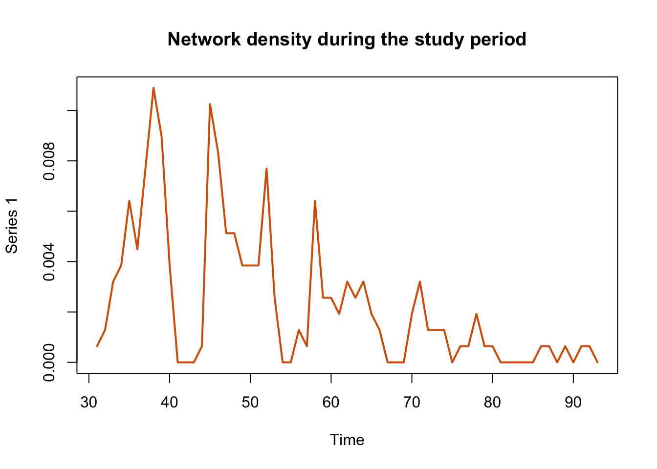
In the previous plot we can see that the activity of movements is bigger at the beginning of the time series and slowly decreases over time until reaching approximately zero.
The function tSnaStats() also allows us to use arguments
to define specific periods of time from which we want to calculate the
statistics
tSnaStats(n1, snafun = "grecip", start = 30, end = 60) %>%
  plot(main = "Network Reciprocity during the interval 30-60", col = colpal[3], lwd = 2)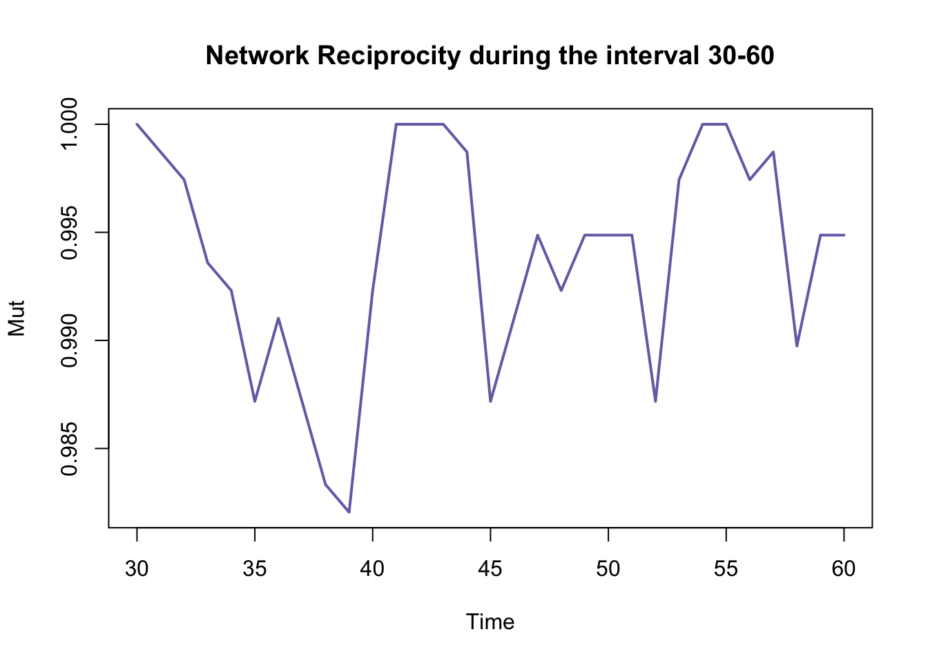
We can also see node-level statistics (e.g. betweenness) using the next function.
apply(tSnaStats(n1, snafun = "betweenness"), 1, mean) %>%
  plot(type = "l", lwd = 2, col = colpal[4])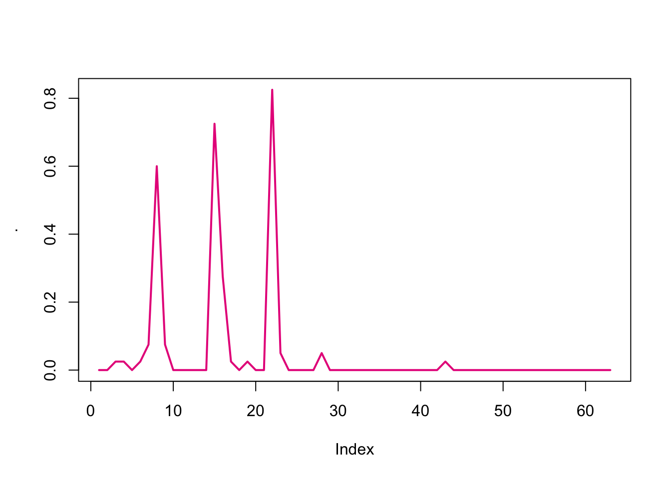
3 Plotting the network
We can use the function plot() to see the network
object, but we can only see the static network because we are not
defining any time interval
plot(n1,mode="kamadakawai") 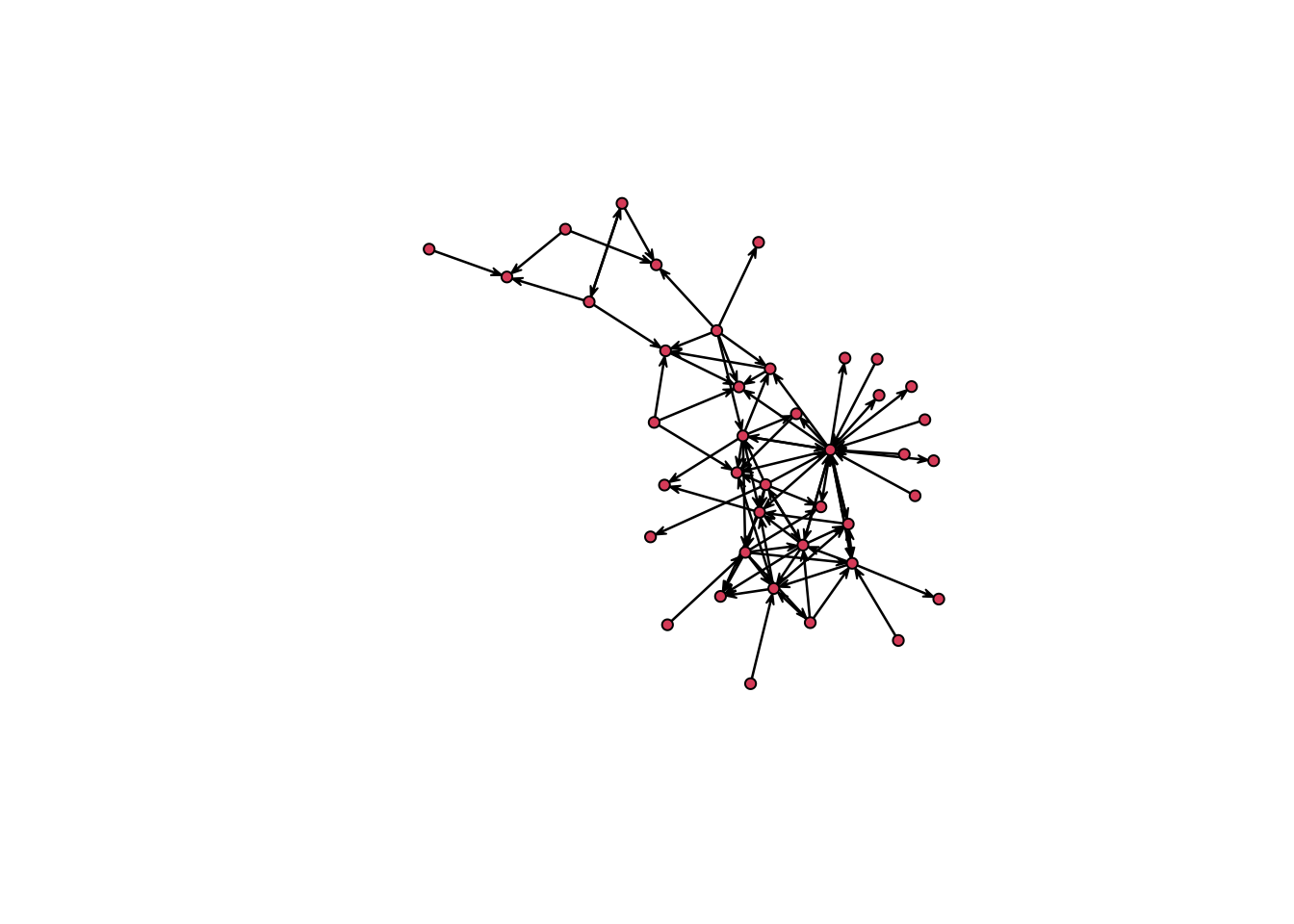
If we want to see a specific period of time, we need to define it.
For this, we can use the function network.extract() to
extract a specific period in the network and then use
plot() to show this extract.
# Plot an interval of time
n1 %>%
  network.extract(onset = 1, terminus = 60) %>%
  plot()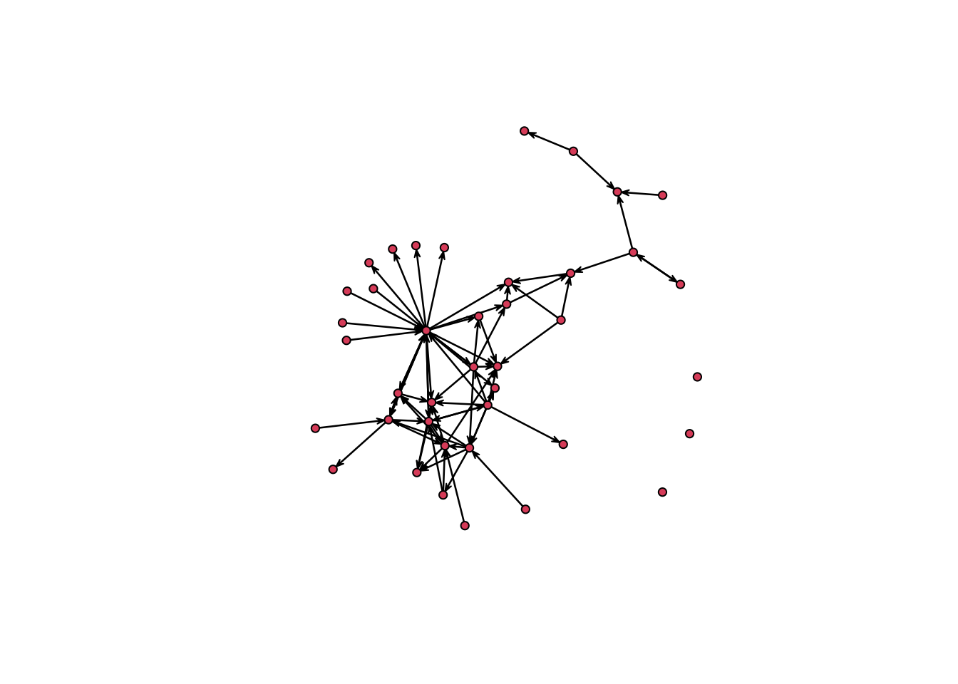
# Plot a specific timepoint and remove isolates
n1 %>%
  network.extract(at = 35) %>%
  plot(displayisolates = F)
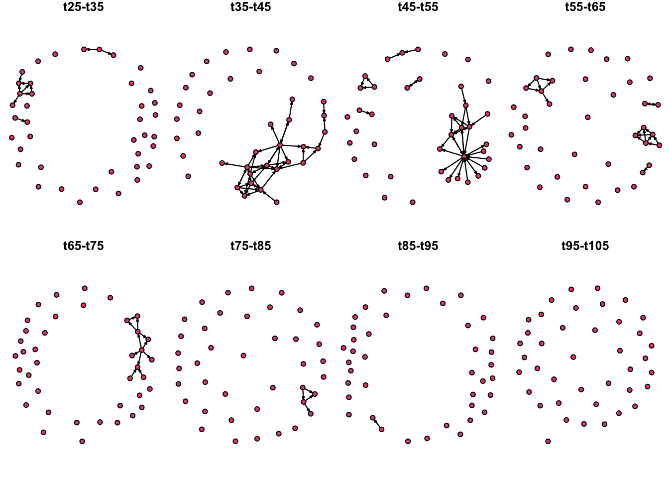
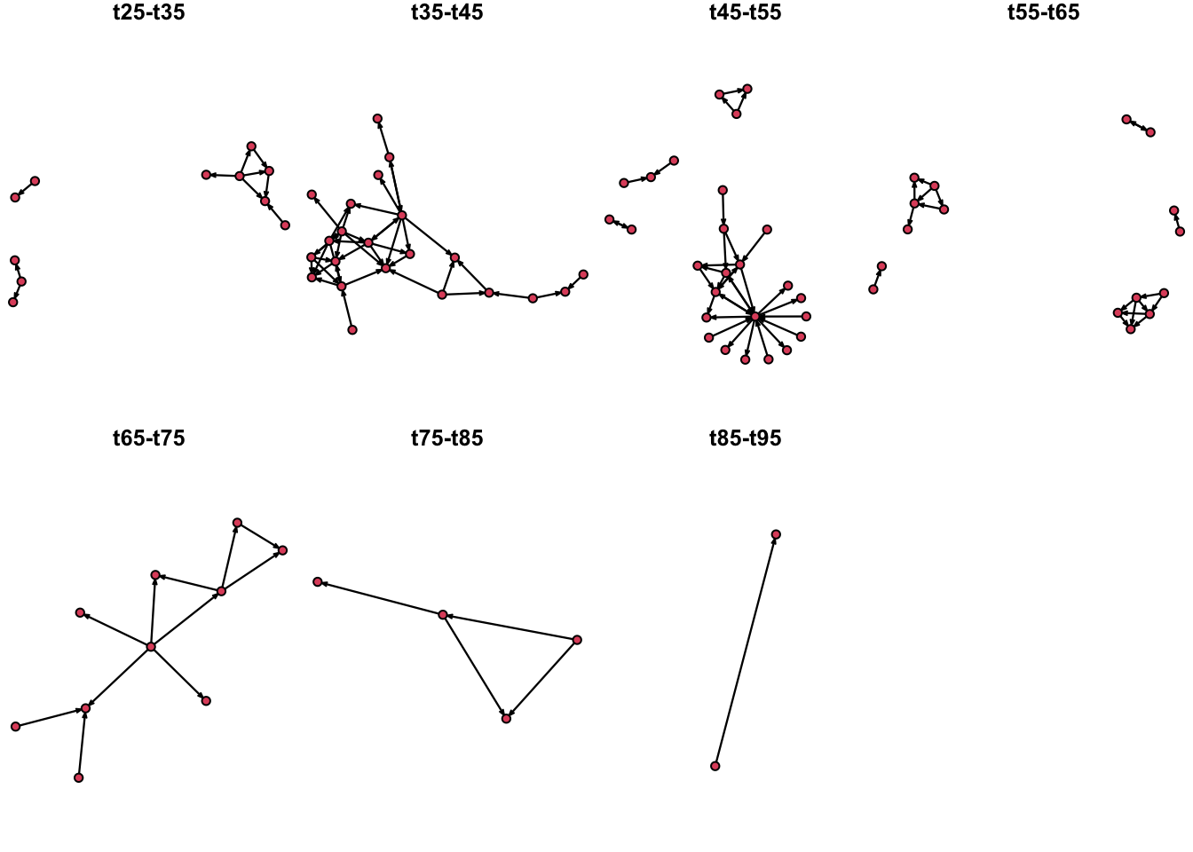
Now we are going to create a plot with multiple periods of time
# First we create a function to plot the network extract we want:
plot.extract <- function(n, onset, terminus, displayisolates = T){
  n %>% # The input network
    network.extract(onset = onset, terminus = terminus) %>% #Extract the time interval
    plot(vertex.cex = 1.5, main = paste0("t", onset, "-", "t", terminus), displayisolates = displayisolates) #Plot the network
}

# Then we define out time intervals
O <- seq(from = 25, to = 95, by = 10)
# We set the layout we want for the plot:
par(mfrow = c(2,4), mar = c(0,0,1,0))
# We use a for loop to plot the network at the defined time intervals.
for(i in O){
  plot.extract(n1, onset = i, terminus = i + 10)
}
We can also use remove the isolates from our visualization to highlight the active nodes, since the last time step (t95-105) had no edges, we will omit this from out time series:
# Then we define out time intervals
O <- seq(from = 25, to = 85, by = 10)
# We set the layout we want for the plot:
par(mfrow = c(2,4), mar = c(0,0,1,0))
# We use a for loop to plot the network at the defined time intervals.
for(i in O){
  plot.extract(n1, onset = i, terminus = i + 10, displayisolates = F) # Notice we added the argument displayisolates = F to remove the isolates
}
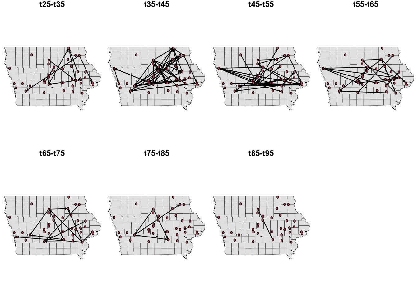
We can use different layouts to plot the extracts of the network. Now, we are going to plot the nodes in their spatial location. For this, we will have to make a little modification of our previous function so we can add the coordinates.
# We set fixed coordinates from the longitude and latitude
a <- as.matrix(node_attrib[, c("long", "lat")])


# Modify the function:
plot.extract <- function(n, onset, terminus, Bg){
  plot(Bg, col = "grey90", lwd = 0.3, main = paste0("t", onset, "-", "t", terminus))
  n %>% # The input network
    network.extract(onset = onset, terminus = terminus) %>% #Extract the time interval
    plot(vertex.cex = 1, coord=as.matrix(a), new = F) #Plot the network
}


# We set the layout we want for the plot:
par(mfrow = c(2,4), mar = c(0,0,1,0))
# We use a foor loop to plot the network at the defined time intervals.
for(i in O){
  plot.extract(n1, onset = i, terminus = i + 10, Bg = IO$geometry)
}
4 Temporally reachable sets
The reachability of a farm help us to identify important nodes in the network that may have a key role in the disease spread. Forward reachability (“fwd”) refers to all the nodes than can be reached from a given node \(v_i\) and backward reachability (“bkwd”) refers to those nodes that reach a given node \(v_i\). We can visualize the distribution of the forward and backward reachability using boxplots
fwd <- tReach(n1, "fwd")
bwd <- tReach(n1, "bkwd")
par(mar=c(2,4,2,2))
boxplot(fwd, bwd, col = "lightgreen", horizontal = T, yaxt = 'n', main = "Reachability of farms")
axis(2, at = c(1,2), labels = c("Fwd", "Bwd"), las=2, lty = 0)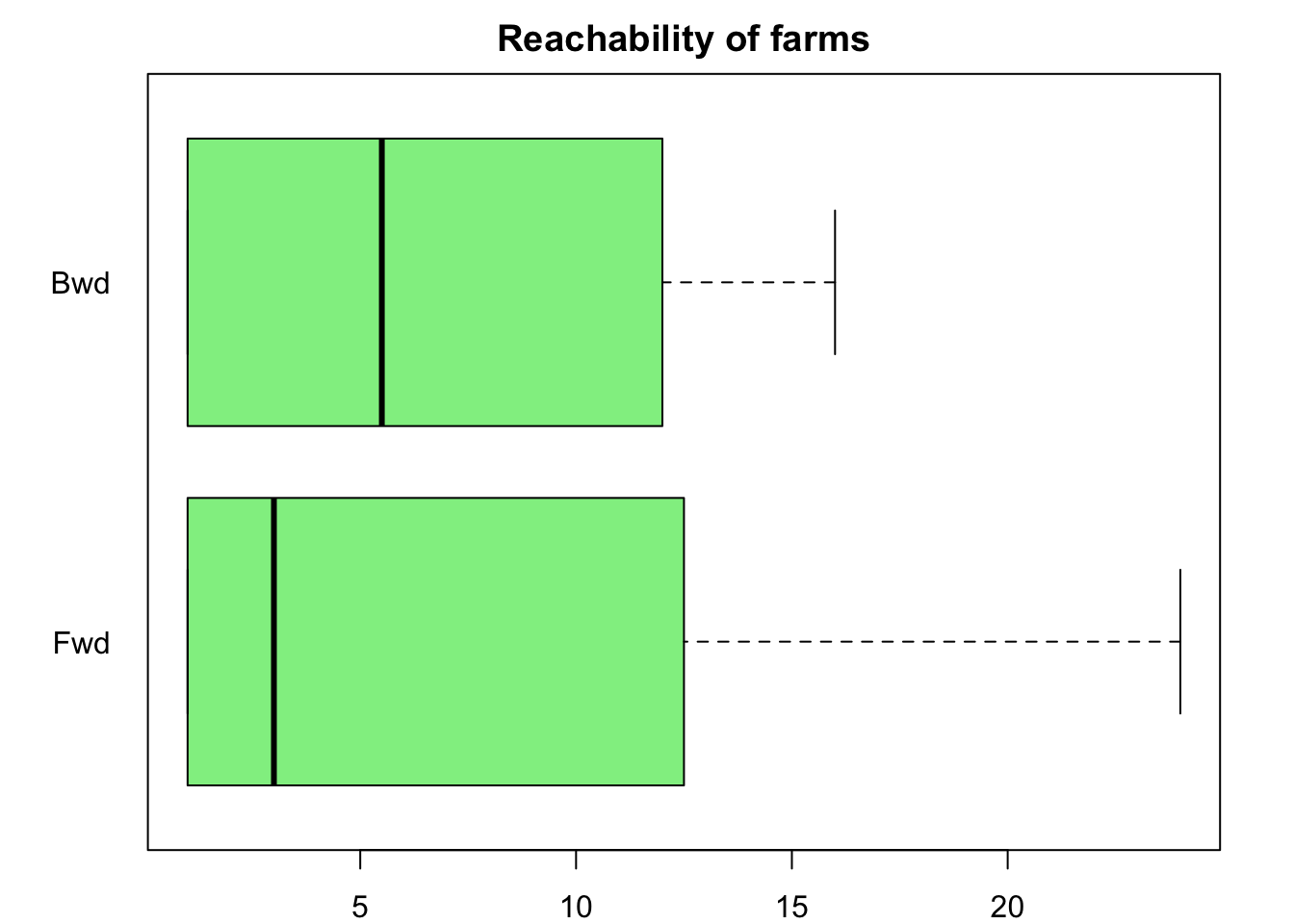
We can also use a dot plot to explore whether any interesting relationship between both types of reachability exists.
plot(fwd, bwd, xlab = "Fwd", ylab = "Bwd", pch = 16, col = rgb(0, 155, 50, max=255, alpha=100))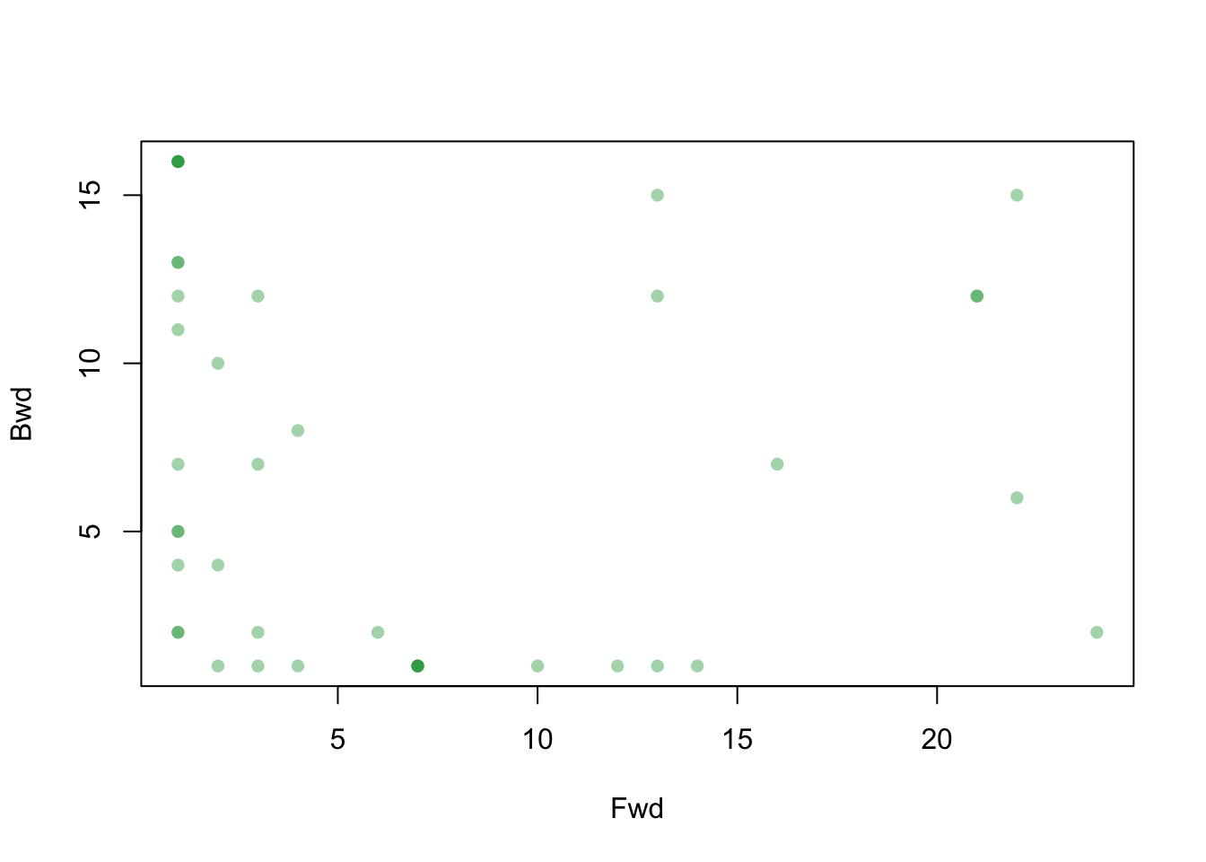
Now, let’s have a look at the farms with the highest forward reachability:
data.frame(id = 1:length(fwd), fwd, bwd) %>%
  arrange(desc(fwd)) %>%
  head(10)
## id fwd bwd
## 1 7 24 2
## 2 8 22 6
## 3 17 22 15
## 4 4 21 12
## 5 14 21 12
## 6 12 16 7
## 7 22 14 1
## 8 1 13 12
## 9 19 13 15
## 10 26 13 1It looks like node (“id”) 7 presents the highest number of reachable farms.
We can visualize the reachable set using the functions
tpath and transmissionTimeline. Both of them
provide the node id and the time when the contact happened. The first
function allow us to visualize the nodes spatially and the second one
shows them in a nice timeline. Let’s start with the first one.
P17 <- tPath(n1, 17, direction = "fwd")
plot(P17)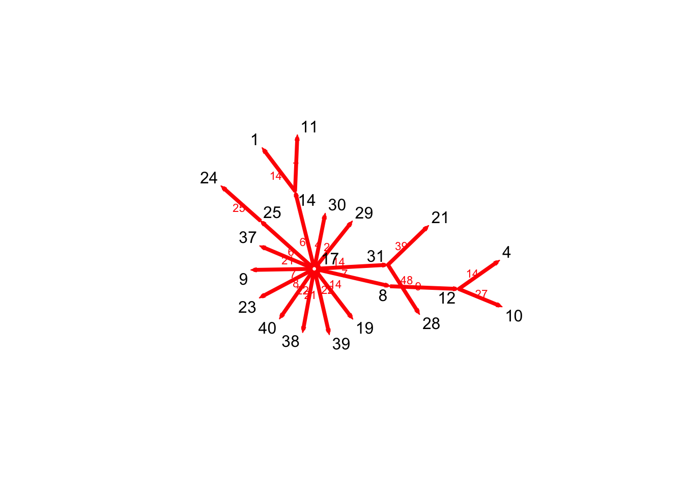
We can also visualize the paths in the full network.
plotPaths(n1, P17, vertex.col = colpal[1], label.cex = 0.5, vertex.cex = 2)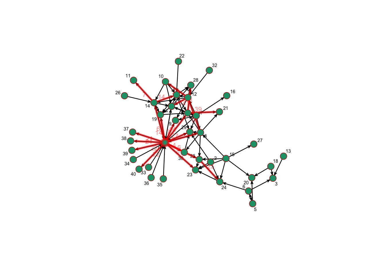
A better way to visualize the paths trough the time period is using
the function transmissionTimeline(). In this visualization,
the x axis represents the time when the event happened and the y axis
represents the generation or steps that happened to reach that node
transmissionTimeline(P17,jitter=T,
          main='Earliest forward path from vertex 17')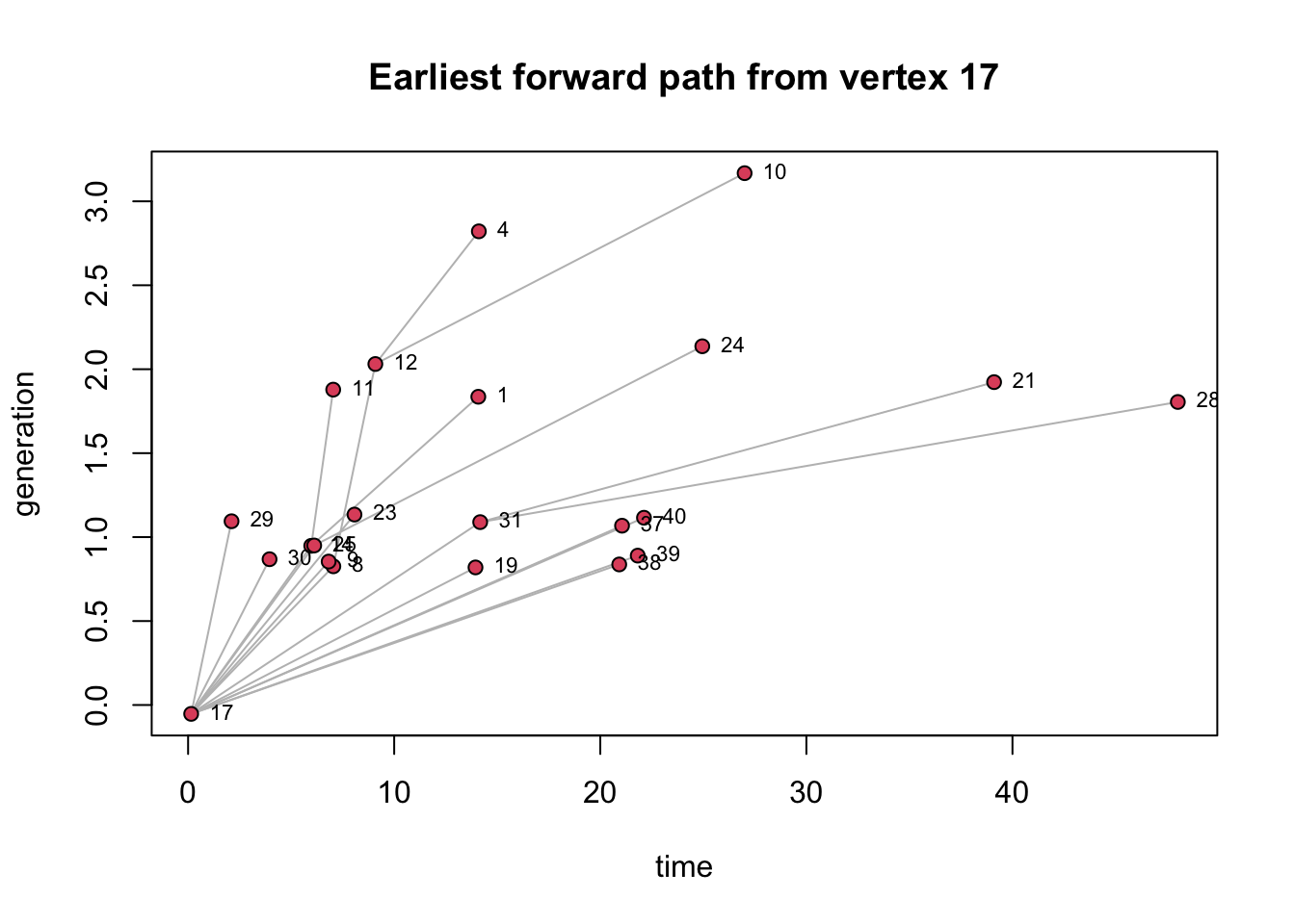
We can also see the backward reachability, which represents the set of nodes that reach a specific node over a time period.
P17 <- tPath(n1, 17, direction = "bkwd", type = "latest.depart")
plot(P17, edge.col = colpal[3])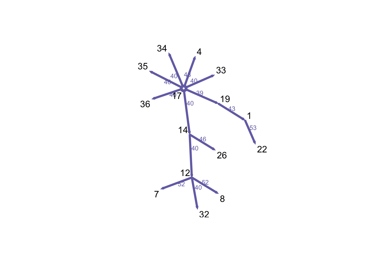
Now we will create a function to show the paths in a spatial and non-spatial plot.
MaPaths <- function(Net, v, direction, Pts, coords, BG){
  # Settings for the visualization arrangement:
  par(mfrow = c(1,2), oma = c(0, 0, 2, 0), mar = c(1, 1, 1, 1))
  # Geth the path for the node we want
  P1 <- tPath(Net, v = v, direction = direction)
  # Plot the map that will be used for background
  plot(BG, col = "grey90", lwd = 0.3, axes = F)
  # add the farm locations:
  points(Pts[, c("long", "lat")], pch = 16, cex = 0.5, col = rgb(0, 150, 100, max = 255, alpha = 50))
  # add the edges to the map
  plot(P1, coord = coords, displaylabels = F, edge.label.col = rgb(0,0,0,0), edge.lwd = 2, vertex.col = "white", edge.col = rgb(0, 200, 50, max=255, alpha=166), new = F)

  # add the edges on the side for a non-spatial visualization
  plot(P1, displaylabels = F,edge.lwd = 2, vertex.col = "white", edge.col = rgb(255, 0, 50, max=255, alpha=166))
  # add the text
  mtext(paste0("Reachable set of farm", v), outer = TRUE, cex = 1.5)
}

MaPaths(Net = n1, v = 17, direction = "fwd", Pts = node_attrib, coords = a, BG = IO$geometry)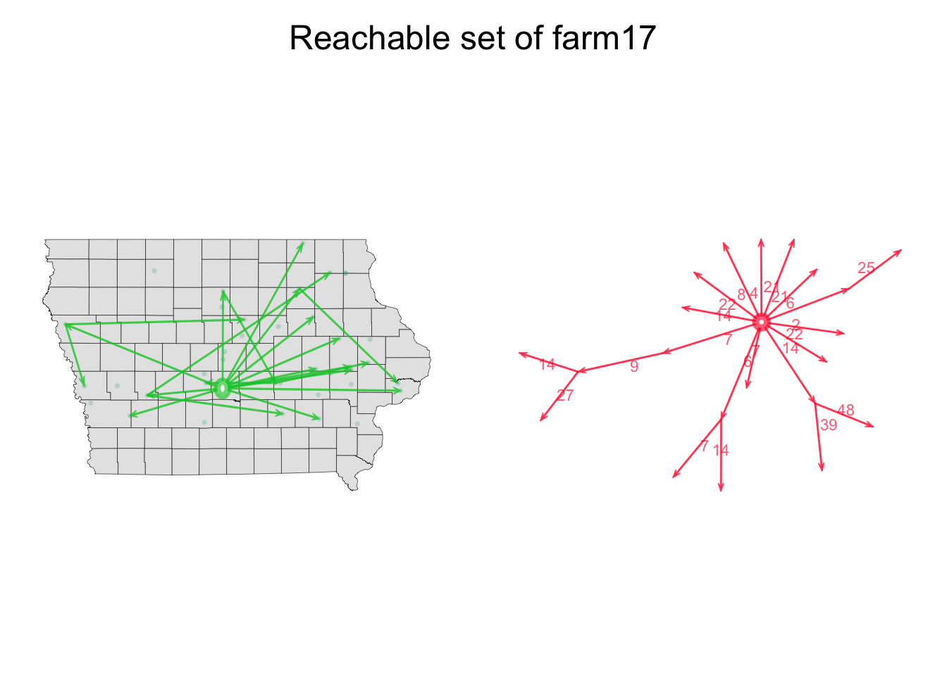
Another way to visualize the network activity is to show the time points when each of the nodes was active. In the following plot, the upper part represents the presence of the node in the network and the lower part represents the activity of the node in the network.
timeline(n1)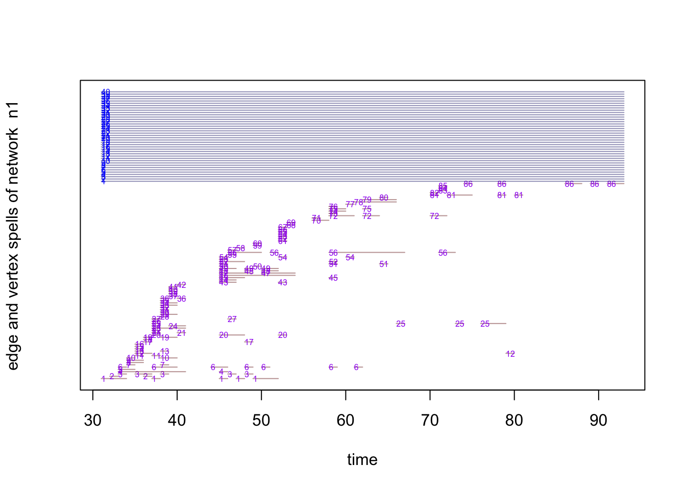
5 Animations
We can also create animations to show the evolution of the contact
patterns over time using the function render.d3movie().
First we will use the function compute.animation() to set
the layout and time frame for the animation.
render.d3movie(n1,
               displaylabels=F,
               launchBrowser = T,
               vertex.cex = scales::rescale(degree(n1), to = c(1, 5)), filename = "Animation01.html")
If we would like to take specific frames for the animation, we can
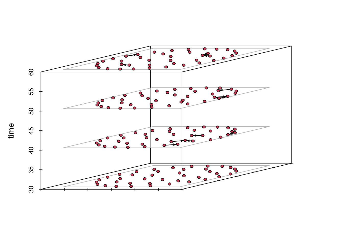
show them stacked in a plot using the function timePrism().
This visualization method works better for small networks.
# Define the intervals
compute.animation(n1, animation.mode = "kamadakawai",
                  slice.par=list(start=30, end=100, interval=1,
                         aggregate.dur=1, rule='any'))

timePrism(n1, at = c(30, 40, 50, 60), planes = T)