In this section we will use a different dataset which consist on GPS locations of 3 different species.
We will define our contact network based on proximity between two animals from the GPS location records.

1 Exploratory analysis

# libraries we will use
library(dplyr) # for data manipulation
library(sf) # For spatial data manipulation
library(sp) # for spatial data
library(ggplot2) # for making figures
library(purrr) # for network transformation
library(tidygraph) # for network manipulation
library(ggraph) # for plotting networks
# We get the data from the STNet package
GPSc <- STNet::GPSc

First we will see how many locations were recorded during the observation period by species:

GPSc %>% 
  count(species_type) # count by species

##   species_type     n
## 1       cattle  9309
## 2         deer 11511
## 3          pig  4428

Now lets create a dataset for the nodes.

Nodes <- GPSc %>% 
  mutate(CollarID = as.character(CollarID)) %>% # convert to character
  distinct(CollarID, species_type) # unique IDs

1.1 Temporal visualization

Now lets see how does the GPS records varies during the observation period:

Daily <- GPSc %>%
  count(Date, species_type) # Count by species and date

ggplot(data = Daily) + # call ggplot
  geom_line(aes(x = Date, y = n, color = species_type), size = 1) +
  theme_minimal()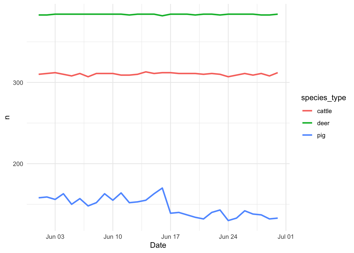

1.2 Spatial distribution of the records

First we will transform our data into a spatial points object.

GPScSP <- GPSc %>%
  st_as_sf(coords = c("X", "Y"), crs = st_crs(4326)) %>% # convert to spatial data
  st_transform(st_crs(32615)) # project the data

Now we use geom_sf() to show the recorded locations on a map.

GPScSP %>% 
  ggplot() + # 
  geom_sf(aes(color = species_type), alpha = 0.2, size = 0.4) +
  theme_minimal() +
  theme(legend.position = 'top')

It looks like the 3 different species have movement ranges where they coincide. To identify where are the species coinciding more often we will use a hexagonal grid.

2 Species range maps

The STNet package includes a function called HexGrid, which creates a hexagonal grid on a spatial field. Here we will use the extent of our points to create the grid.

# First we create a field that represents the study area:
Border <- as(raster::extent(GPScSP), "SpatialPolygons") %>%
  st_as_sf()
# We define the CRS
st_crs(Border) <- st_crs(GPScSP)

# Load the STNet library:
library(STNet)
# We use the HexGrid function:
BorderHex <- HexGrid(cellsize = 500, Shp = Border)

## Warning in proj4string(obj): CRS object has comment, which is lost in output; in tests, see
## https://cran.r-project.org/web/packages/sp/vignettes/CRS_warnings.html

## Warning: use *apply and slot directly

## Warning: use *apply and slot directly

# Plot the grid:
plot(BorderHex$geometry)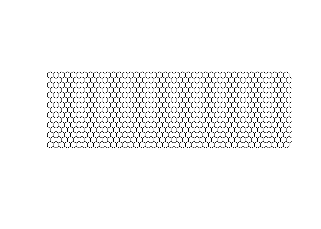

Next we wull use another function from the STNet package that counts the number of points per hexagonal cell. The arguments we need are:

Hex, the hexagonal grid we created.
Points The locations that we want to count. for this function is also necesary to have installed the package sp, so make sure its installed and loaded.

Now lets plot the movement ranges for the species on the observed period:

# For cattle:
GPScSP %>%
  filter(species_type == "cattle") %>% # we filter to only cattle records
  HexMap(Hex = BorderHex, .) %>% # count the points per grid cell
  ggplot(., aes(fill = N)) + # call ggplot
  geom_sf() + # add the spatial layer
  scale_fill_gradient(low="white", high="red") + # define the gradient for the fill
  ggtitle("Cattle Range") + # add a title
  theme_void() #add a theme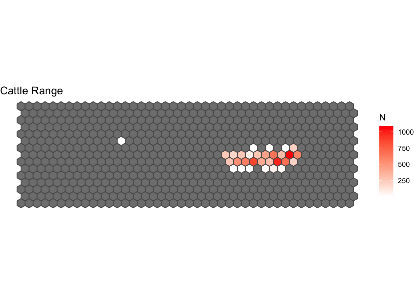

Exercise: Create the range maps for the other 2 species (deer y pig) and use different colors.

3 Defining the network:

3.1 Defining the contacts:

Now we will define our network. We are interested in all the contacts that happened between animals at a distance of < 1 m.

This function might take some time, if you want to skip this part, the data is available inside the STNet package.

# Lets change the names to test the function:
colnames(GPSc)[c(1, 4, 6, 7)] <- c("id", "date", "Longitude", "Latitude")
# Run the function
Edges <- CreateNetwork(DF = GPSc[,], # This is our data
                       DTh = 1, # TTthe distance threshold
                       DateTime = "date", # Name of the variable that indicates the date and time
                       ID = "id", # name of variable for id
                       coords = c("Longitude", "Latitude") # Name of variable for coordinated
                       ) # 14,869

To load the data directly from the STNet package we can use the function:

Edges <- STNet::. %>%  # load the dataset from the package
  mutate_at(.vars = c('Var1', 'Var2'), .funs = as.character) # convert the variables to character

This dataset includes:

Distance: distance between the recorded contact.
DateTime: The time when the contact happened.
Var1 and Var2: nodes involved in the contact. Remember that since these contacts are registerd from the location of the animals, we don’t know who started the contact, so it is not directed.
X.x, Y.x, X.y, Y.y: the spatial location of the nodes at that time.

3.1.1 Contacts between species:

We can also detect areas where the contacts between species are happening.
For this we will create a subset of the data that includes only contacts between different species.

# Add variable for species
Edges <- Edges %>%
  left_join(Nodes, by = c("Var1" = "CollarID")) %>% # Var1 one of the nodes
  rename(Sp1 = species_type) %>%
  left_join(Nodes, by = c("Var2" = "CollarID")) %>% # Var 2 is the other node
  rename(Sp2 = species_type)

InterSp <- Edges %>% 
  filter(Sp1 != Sp2) %>% # select contacts where the species are different
  data.frame()

# we create a projected dataset 
InterSp_sp <- InterSp %>%
  dplyr::select(DateTime, Var1, Var2, Sp1, Sp2, X.x, Y.x) %>%
  st_as_sf(coords = c("X.x", "Y.x"), crs = st_crs(4326)) %>%
  st_transform(st_crs(32615))
  
# Count the observations per grid cell
IspH <- HexMap(BorderHex, Points = InterSp_sp)

# make the figure
ggplot(IspH, aes(fill = N)) +
  geom_sf() +
  scale_fill_gradient(low="white", high="gold3") +
  ggtitle("Contacts between species") +
  theme_void()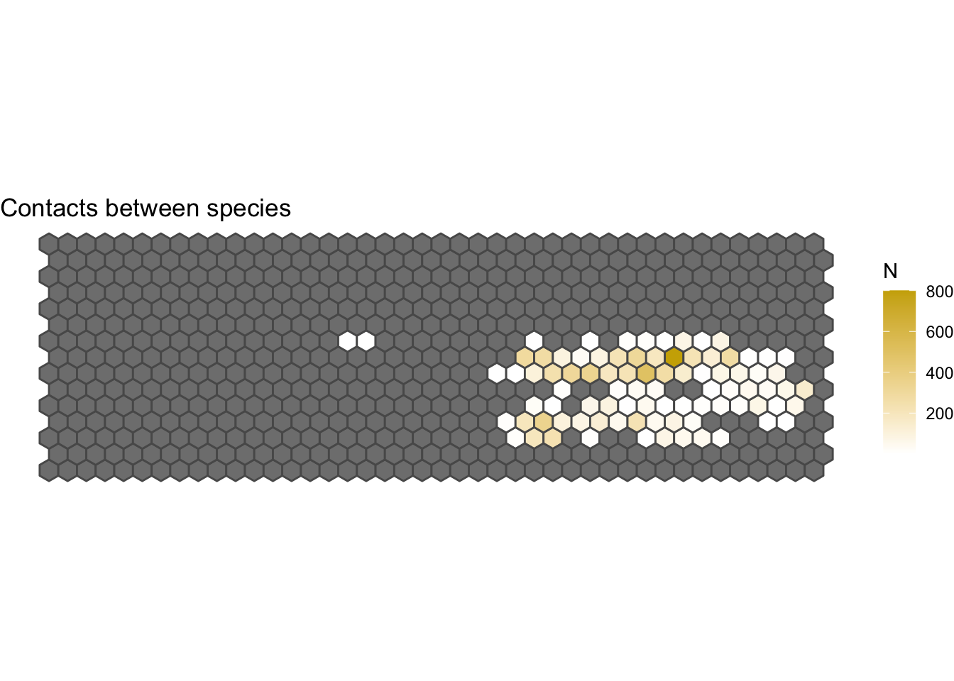

3.2 Define the nodes:

We previously defined the nodes, we can see that there are 36 animals in our network.

Nodes %>%
  count(species_type)

##   species_type  n
## 1       cattle 13
## 2         deer 16
## 3          pig  7

3.3 Creating the network:

# Create the network:
G1 <- as_tbl_graph(Edges[c("Var1", "Var2")], directed = F) %N>% 
  mutate(degree = centrality_degree()) %>% 
  left_join(Nodes, by = c('name' = 'CollarID')) %E>%
  mutate(N = as.integer(1)) %>% # Create a variable to count the number of contact:
  convert(to_simple) %E>%  # now we will convert it to a simple network
  mutate(weight = map_int(.orig_data, ~.x %>% pull(N) %>% sum()))  # We have to sum all the repeated movements

ggraph(graph = G1) +
  geom_edge_link(aes(alpha = weight)) +
  geom_node_point(aes(size = degree), col = 'darkred') +
  scale_size(range = c(0.3, 10)) +
  theme_void()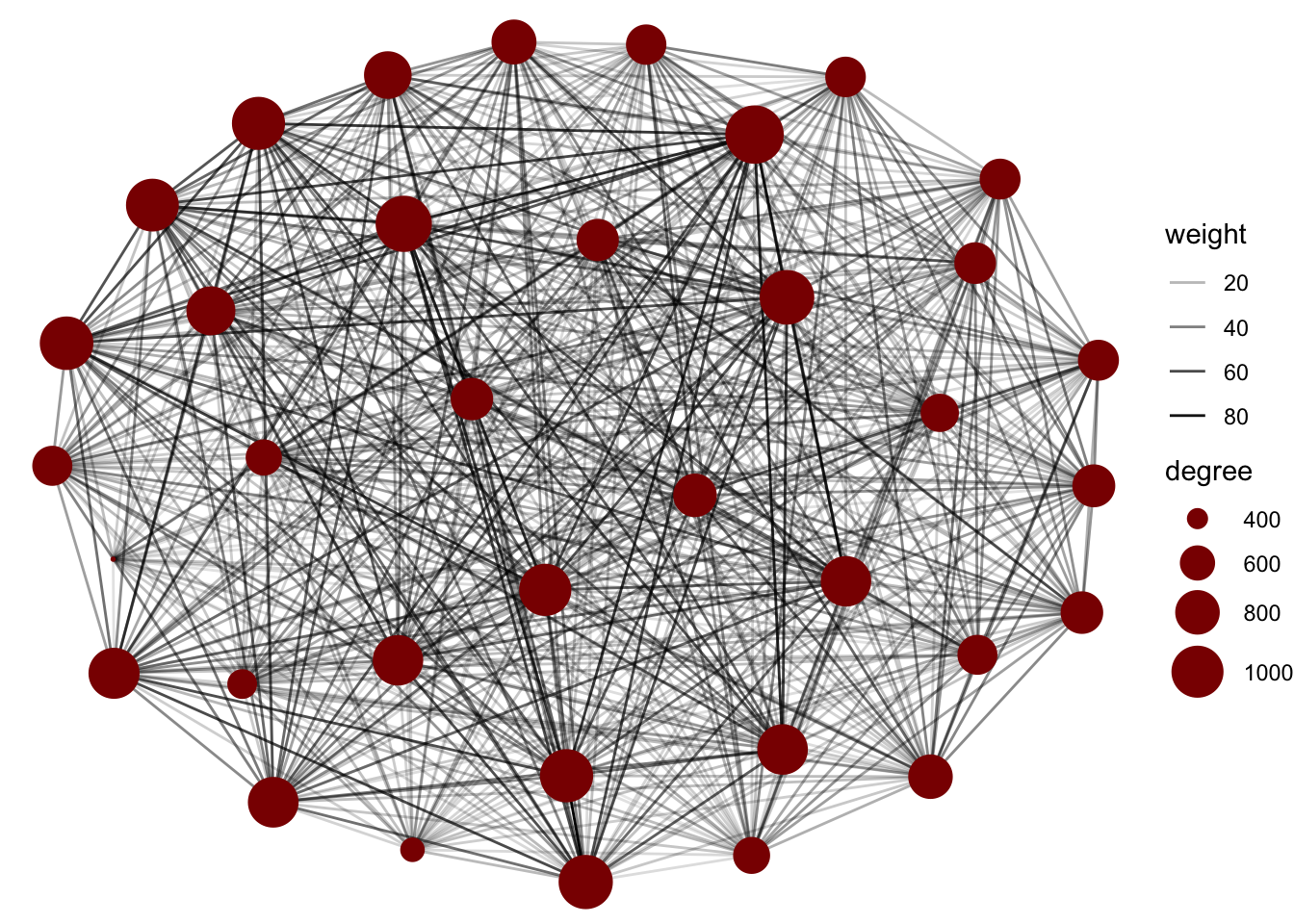

3.4 Networks by species:

We can filter the nodes based on the species type to create a figure of only one species type.

G1 %N>% 
  filter(species_type == 'cattle') %>% 
  ggraph() +
  geom_edge_link(aes(alpha = weight)) +
  geom_node_point(aes(size = degree), col = 'darkgreen') +
  theme_void()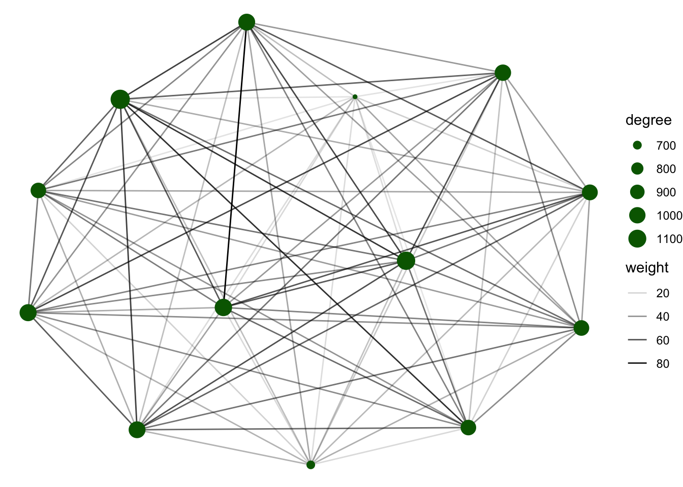

Exercise: create the network for the other 2 species

Lab 3