Day 02
How can we find help with R?
Using the ? operator:
How can we find help with R?
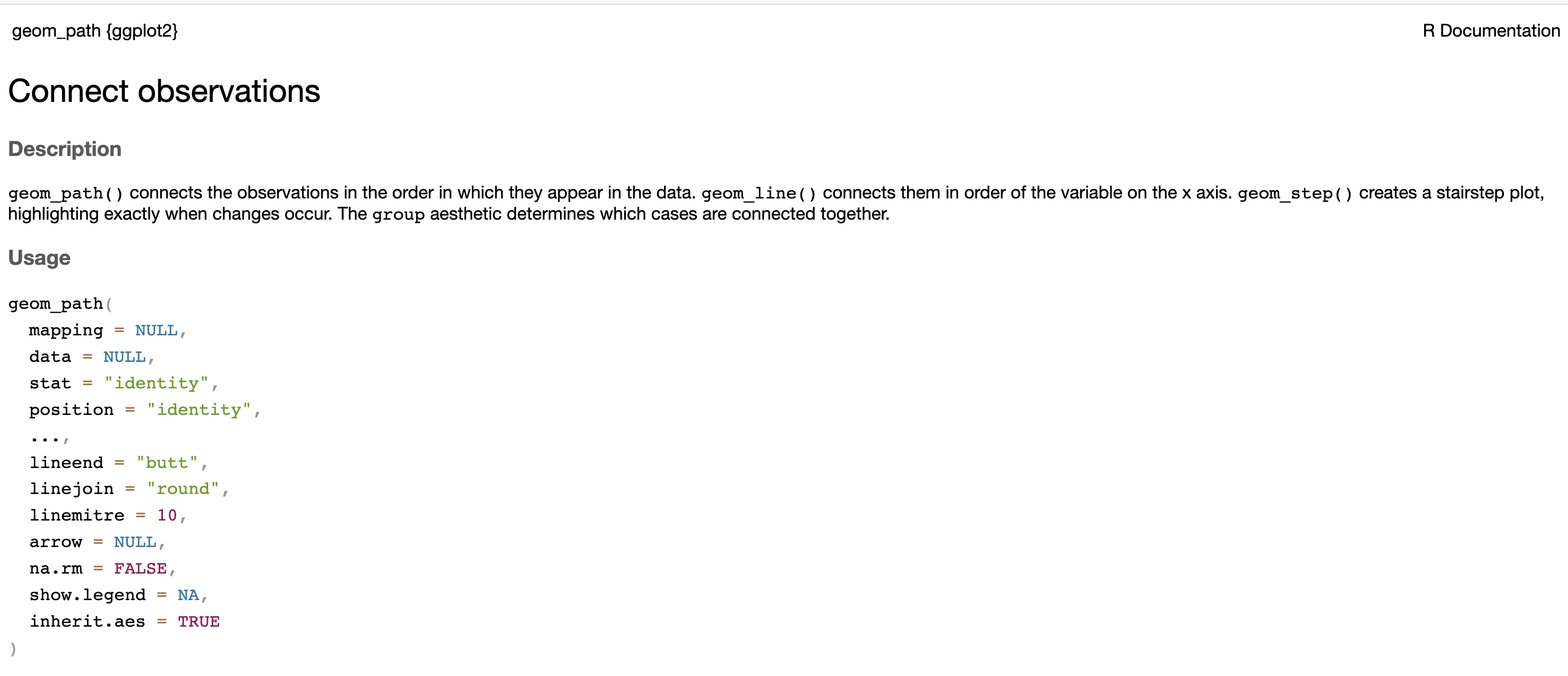
How can we find help with R?
How can we find help with R?
How can we find help with R?

How can we find help with R?

ggplot2
- We build our figures based on layers
- Similar syntax as dplyr
- We can combine data wrangling and visualization into a single code chunk
Instead of the %>%, in ggplot we connect pieces of code with +
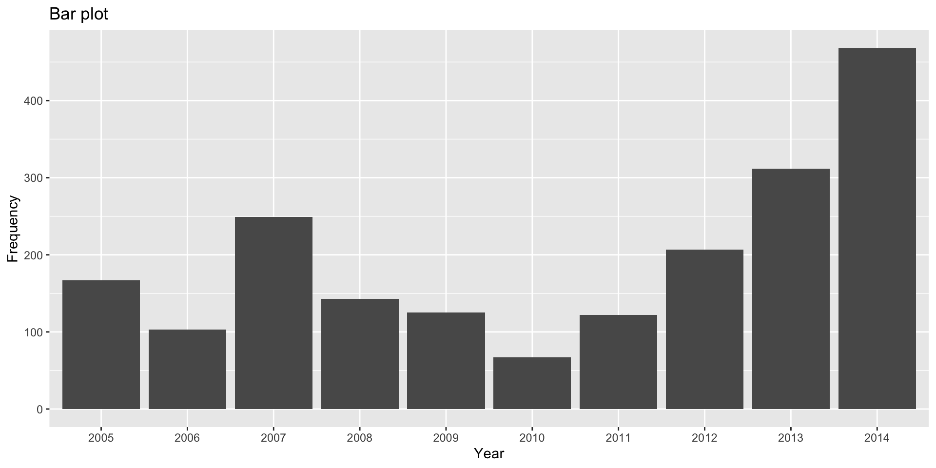
Example

Example
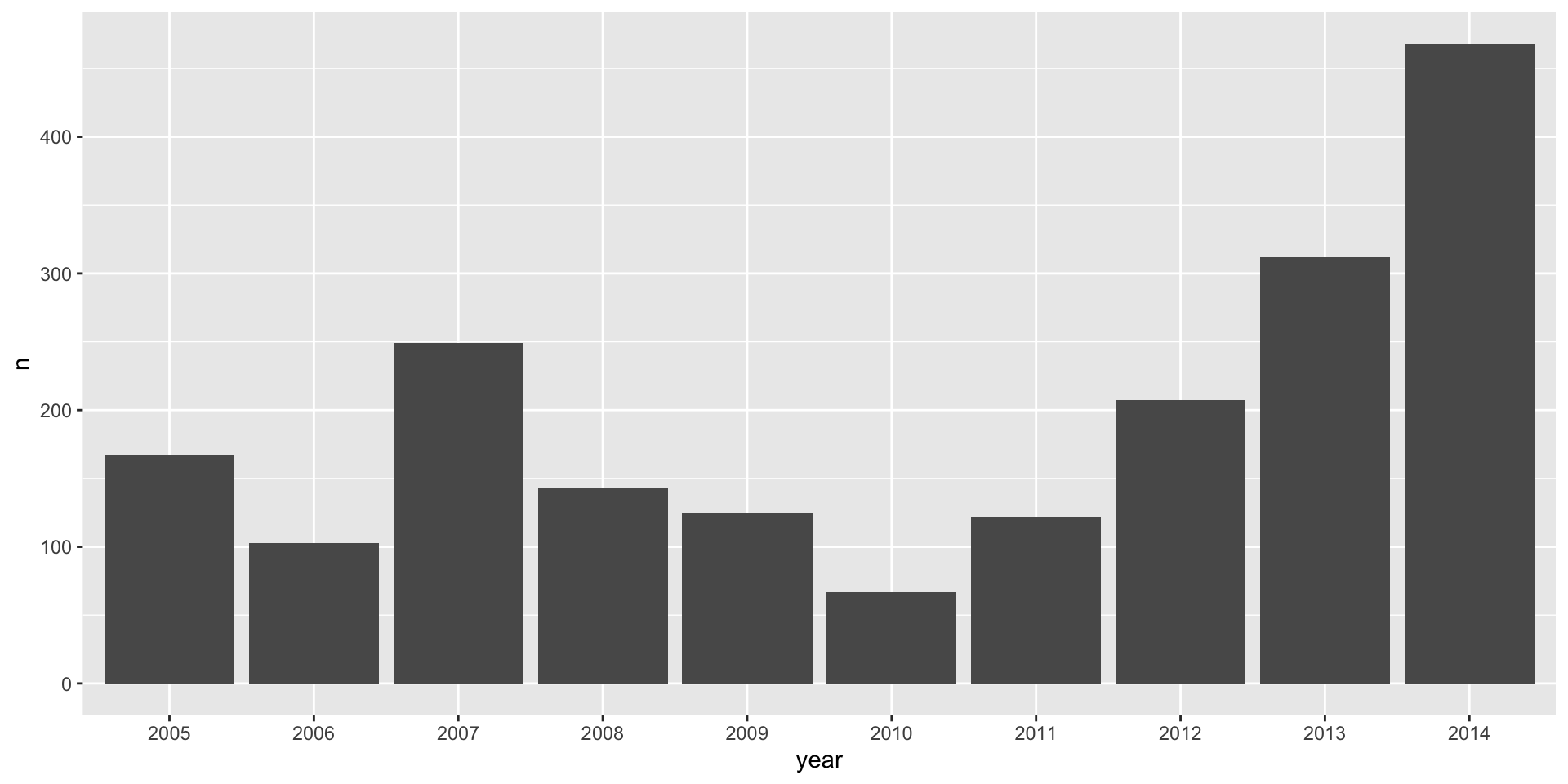
Example
ggplot2

How can we find help with R?
Spatial data formats
Vectors 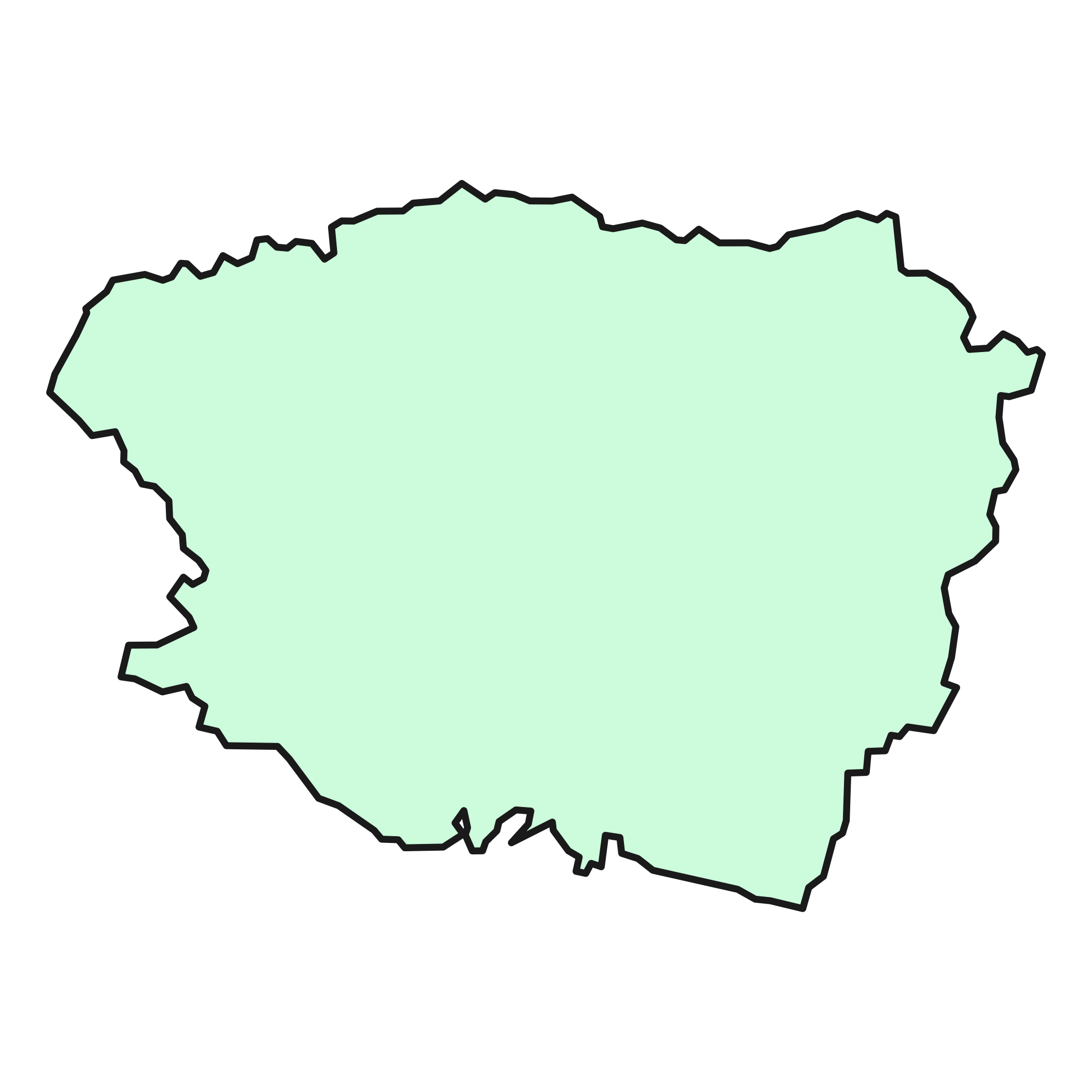
Rasters 
Spatial resolution

Vectors
Point

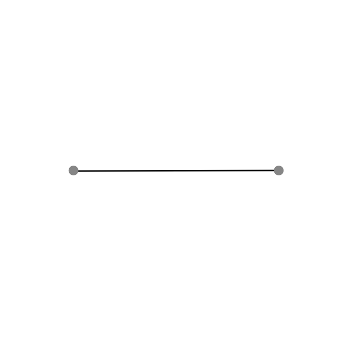
Lines
Polygon

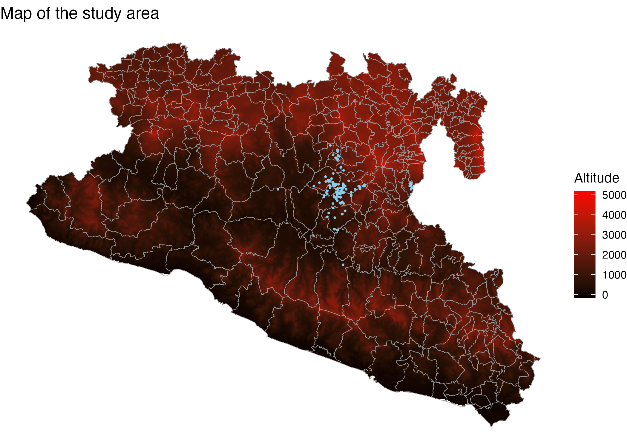
Maps
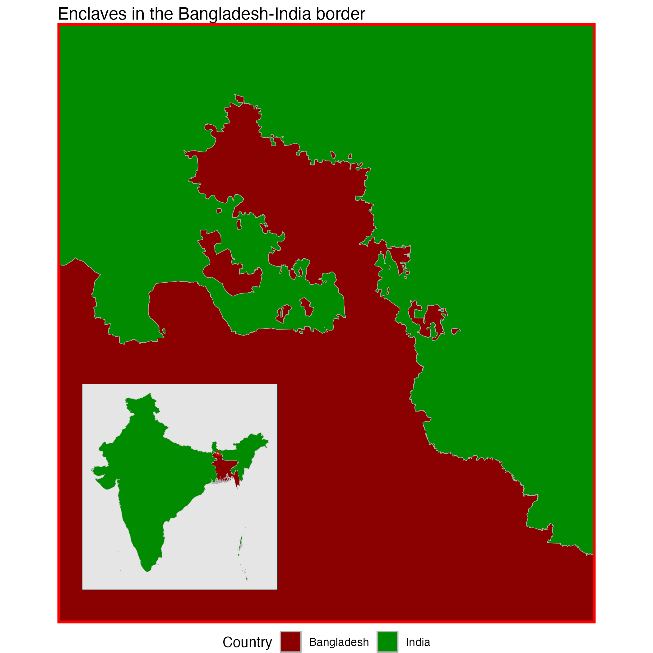
ggplot() + # create the empty canvas
  geom_stars(data = Mxst) + # add raster layer
  geom_sf(data = Area, fill = NA, col = 'grey60') + # add polygon layer
  geom_sf(data = capturesSp, cex = 0.3, col = 'skyblue') + # add point layer
  theme_void() + # theme for the figure
  scale_fill_gradient(low = 'black', high = 'red', na.value = NA) + # color for the gradient
  labs(title = 'Map of the study area', fill = 'Altitude') # labels for the figure