Day-03
Review: Maps
ggplot() + # create the empty canvas
  geom_stars(data = Mxst) + # add raster layer
  geom_sf(data = Area, fill = NA, col = 'grey60') + # add polygon layer
  geom_sf(data = capturesSp, cex = 0.3, col = 'skyblue') + # add point layer
  theme_void() + # theme for the figure
  scale_fill_gradient(low = 'black', high = 'red', na.value = NA) + # color for the gradient
  labs(title = 'Map of the study area', fill = 'Altitude') # labels for the figure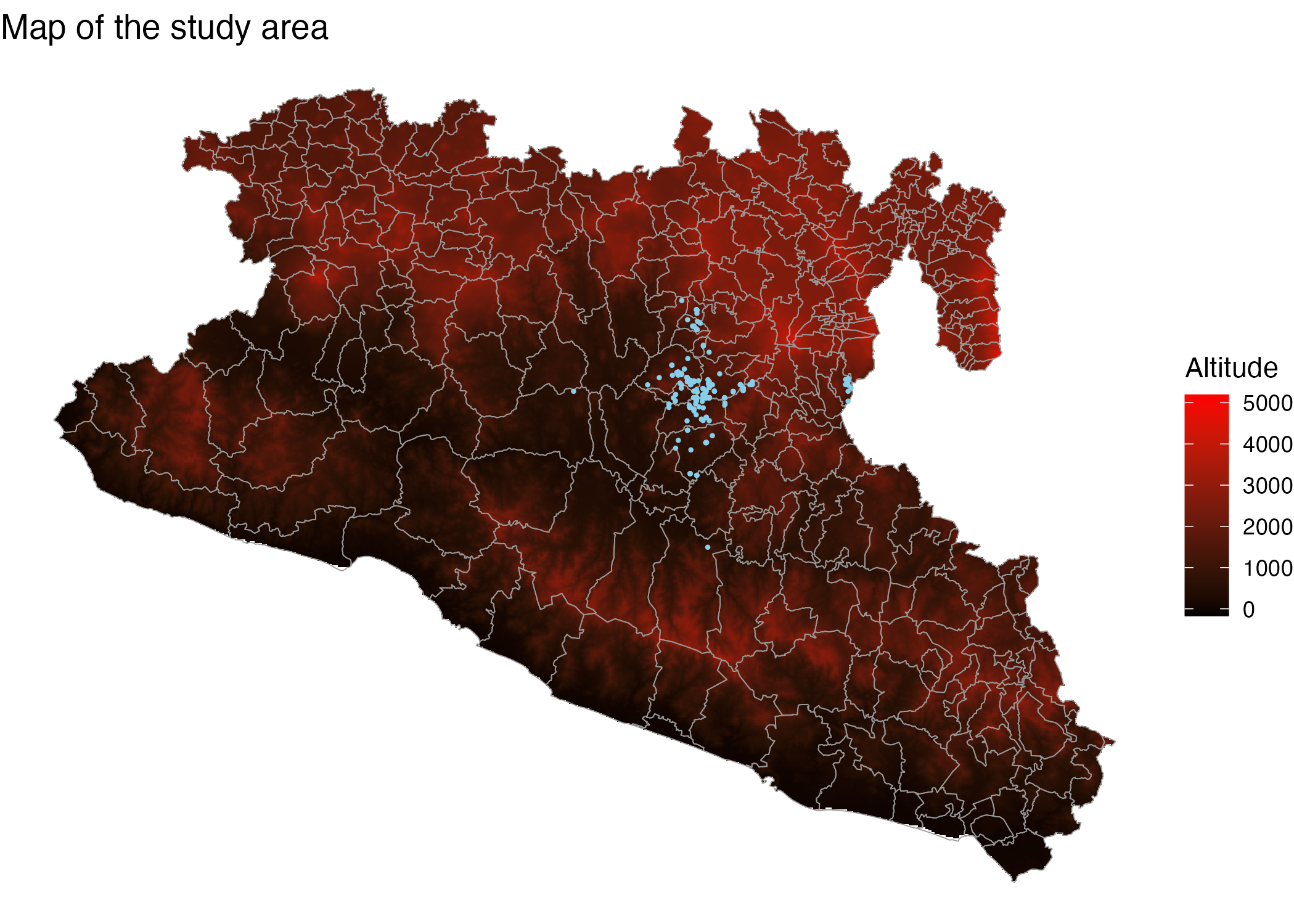
Why represent events in a network?
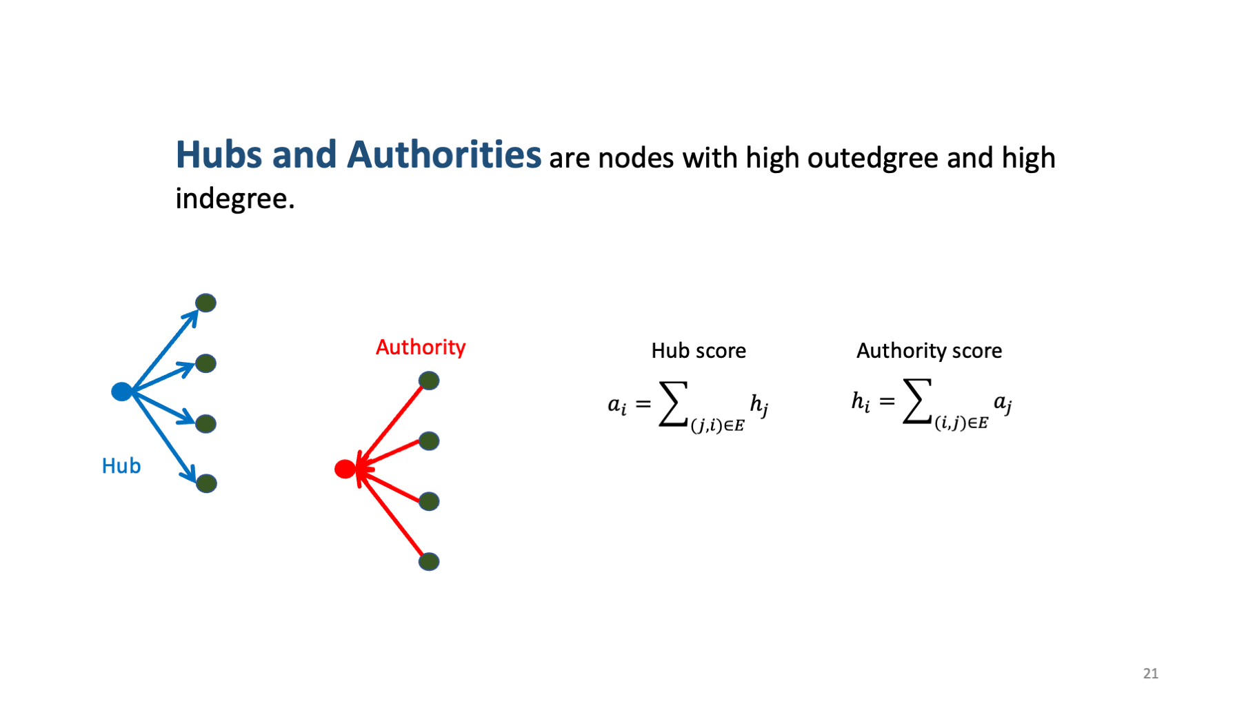
Identify individuals that are very active 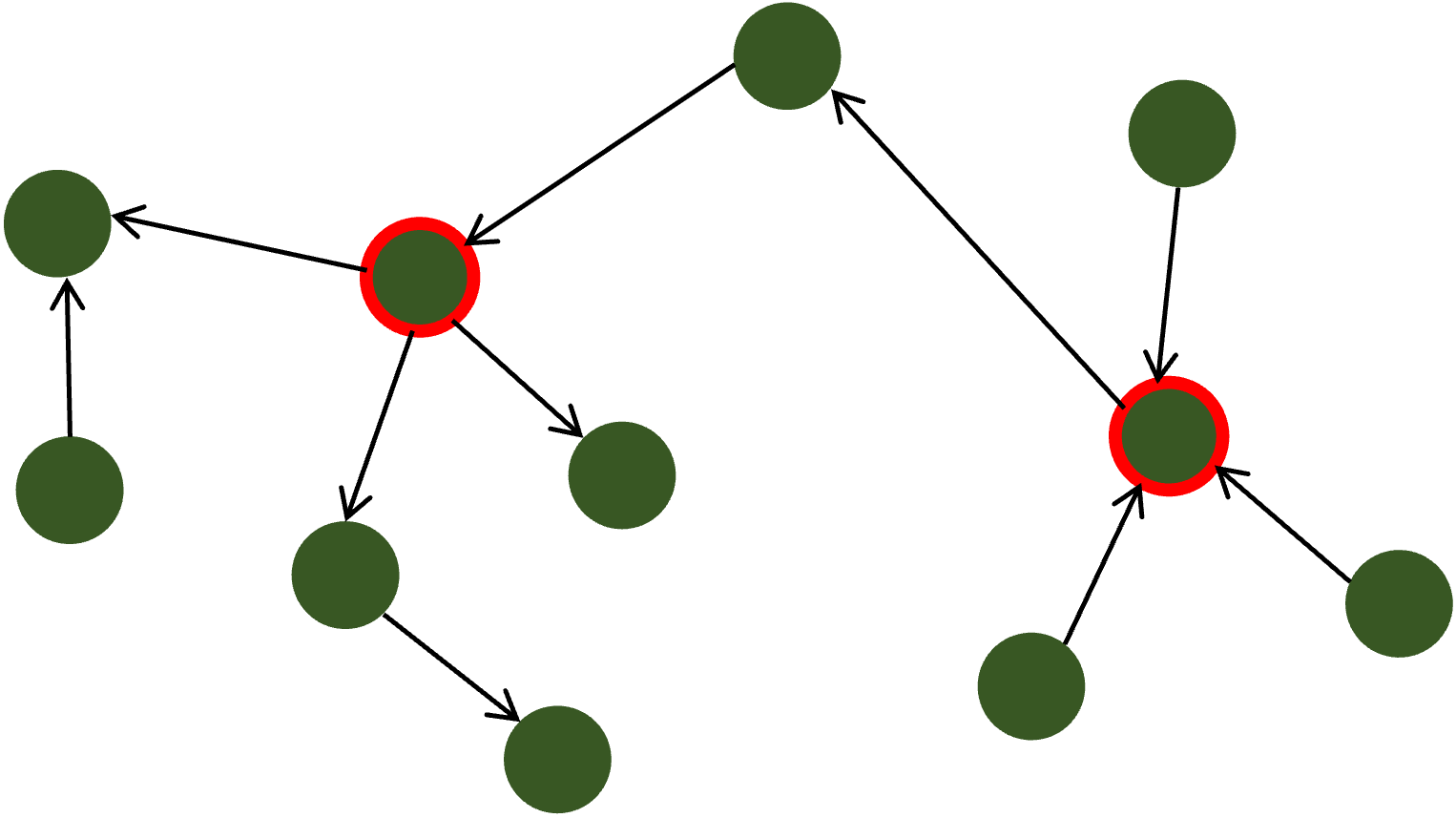
Identify individuals that are intermediate 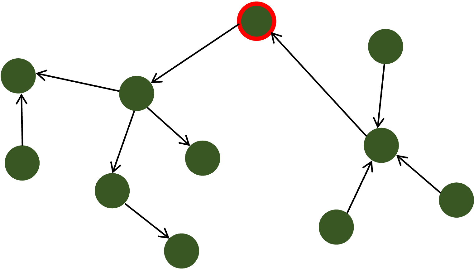
What is a graph?
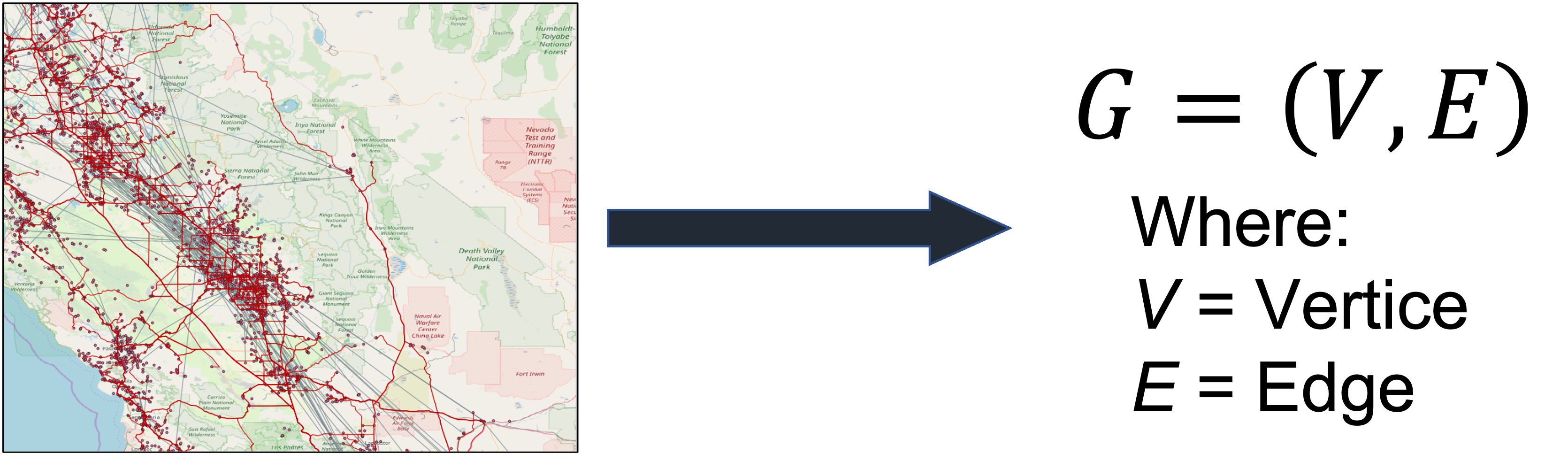
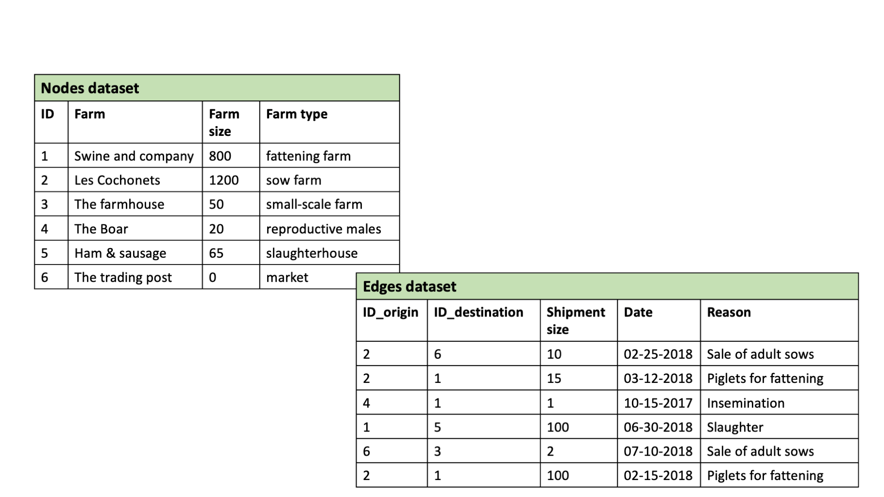
Elements of a network
Nodes (vertices)
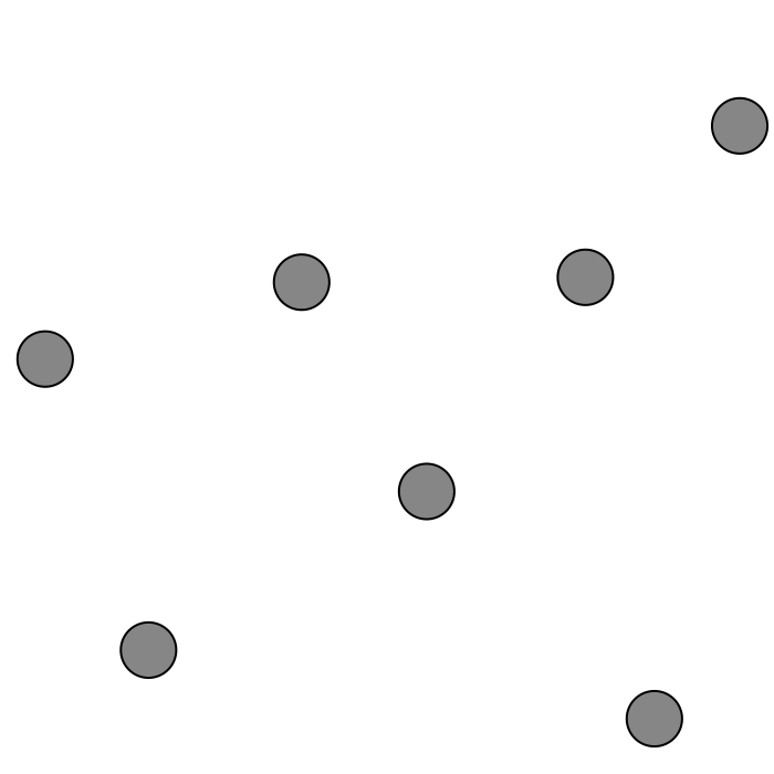
\[V = [1, 2, 3, ..., i]\]
Elements of a network
Nodes (vertices)
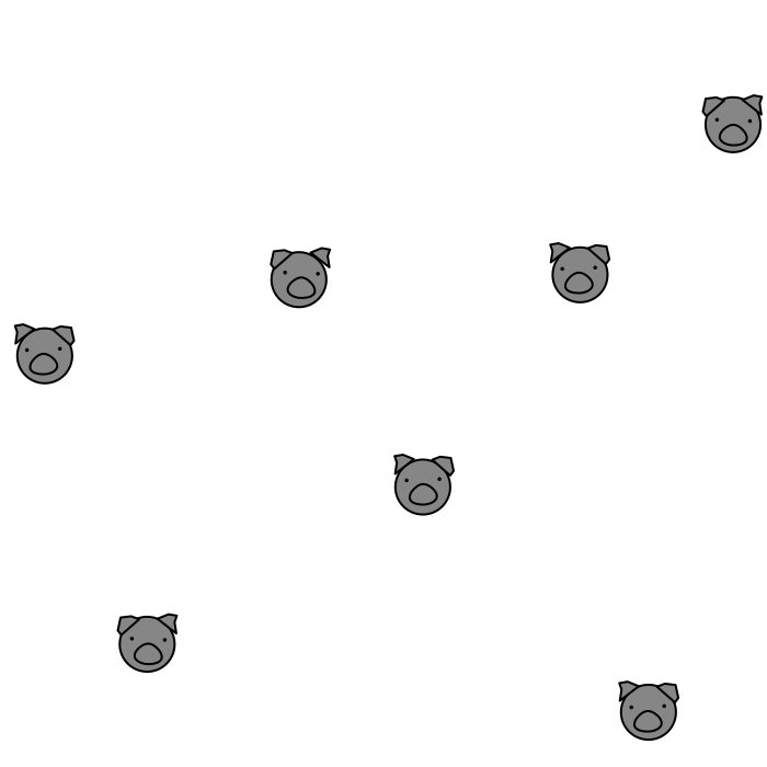
\[V = [1, 2, 3, ..., i]\]
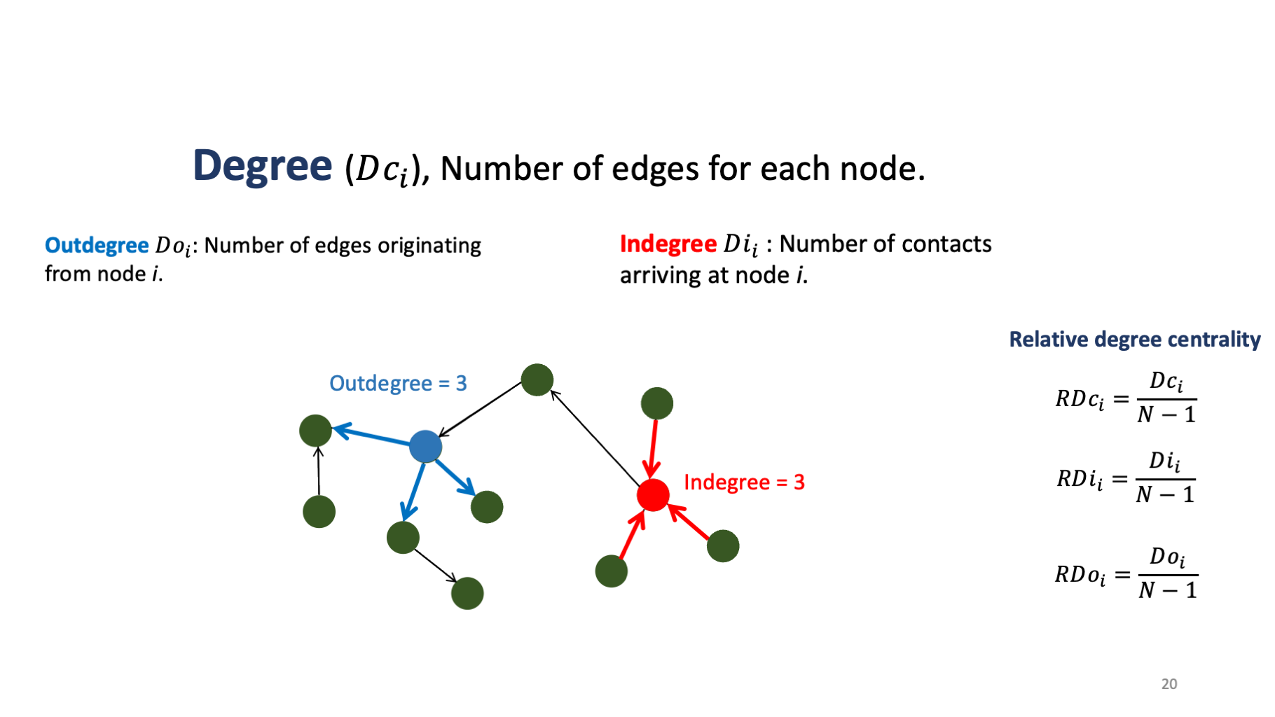
Elements of a network
Edges (links)

\[E = [(1, 2), (1, 3), (2, 3), ..., (i,j)]\]
Elements of a network
Network attributes
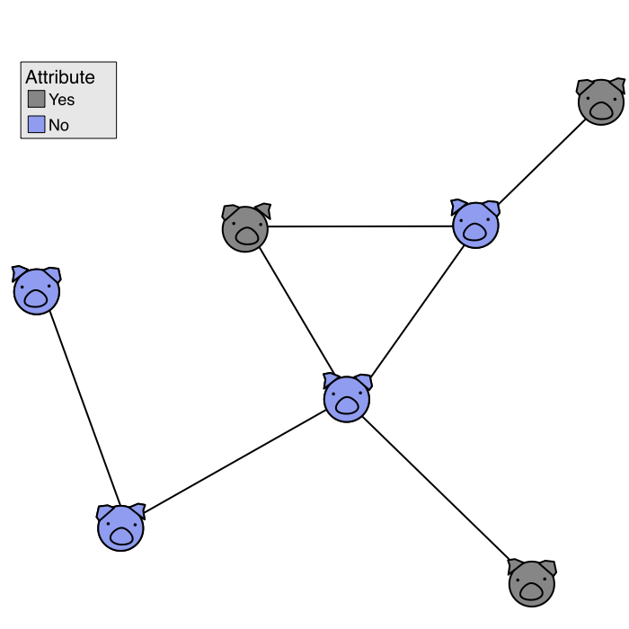
\[V = [0, 1, 1, ..., x_i]\]
Data structure
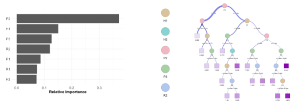
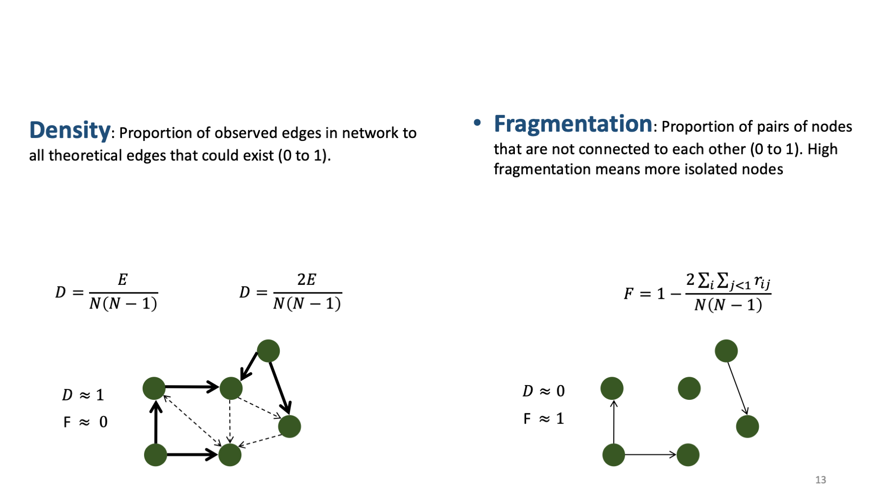
General properties
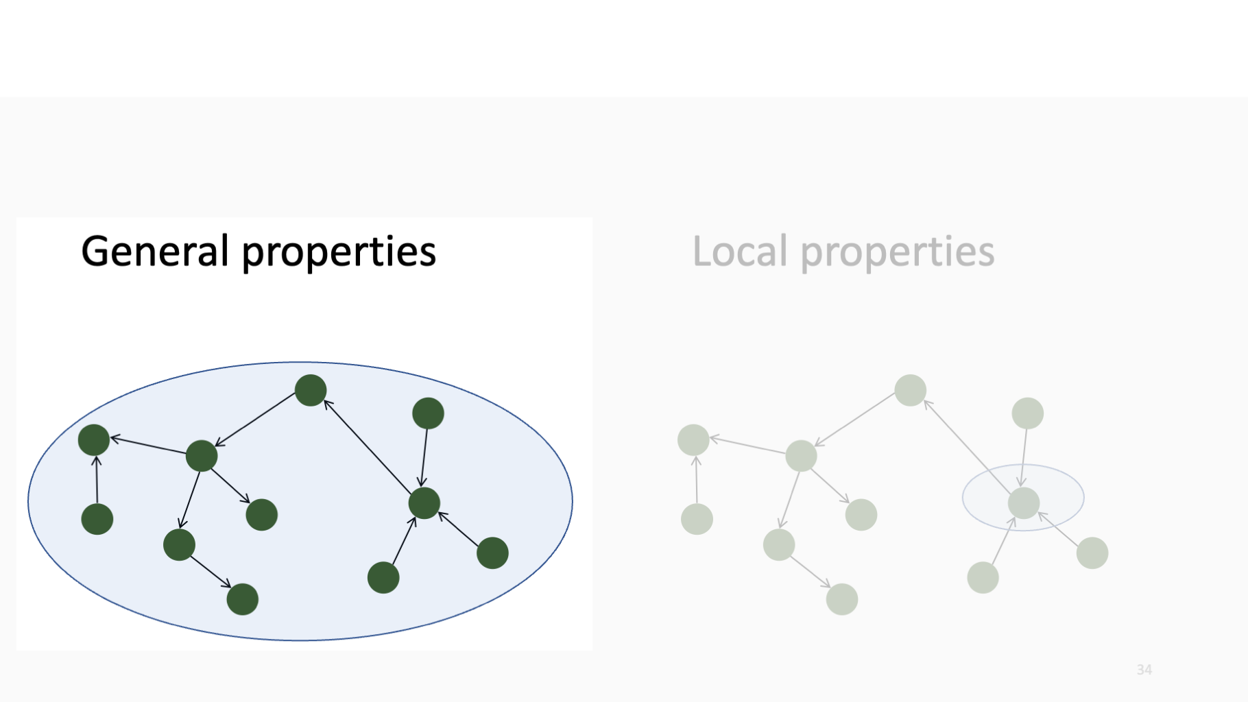
General properties
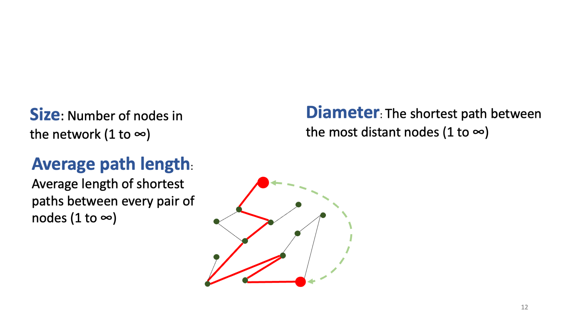
General properties
Local properties
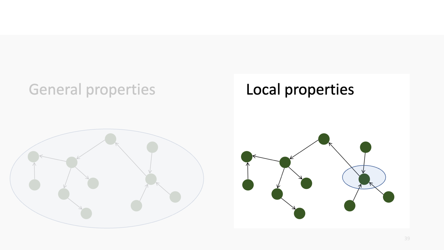
Local properties
Local properties
Visualization
ggraph(net, layout = 'kk') + # this is our empty canvas
  geom_edge_link(aes(width = pigs.moved)) + # Add the edges
  geom_node_point() + # Add the nodes
  scale_edge_width(range = c(0.01, 0.9)) + # we set the range for the width of the edges
  labs(title = 'Title for the plot', edge_width = 'Number of pigs moved') # labels for the figure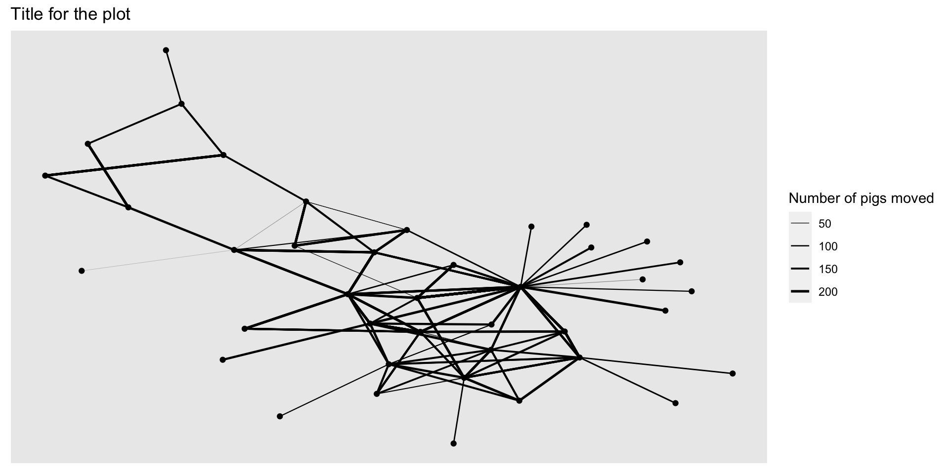
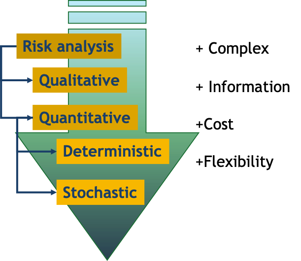
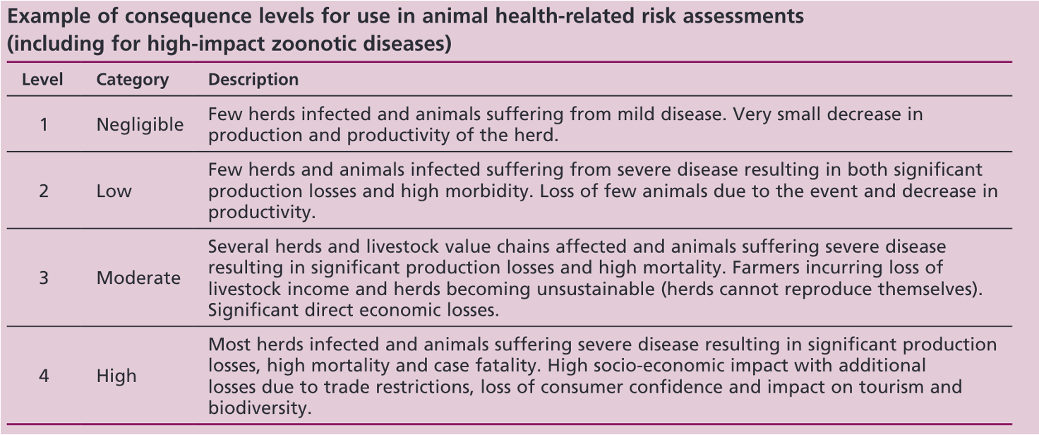
Risk analysis
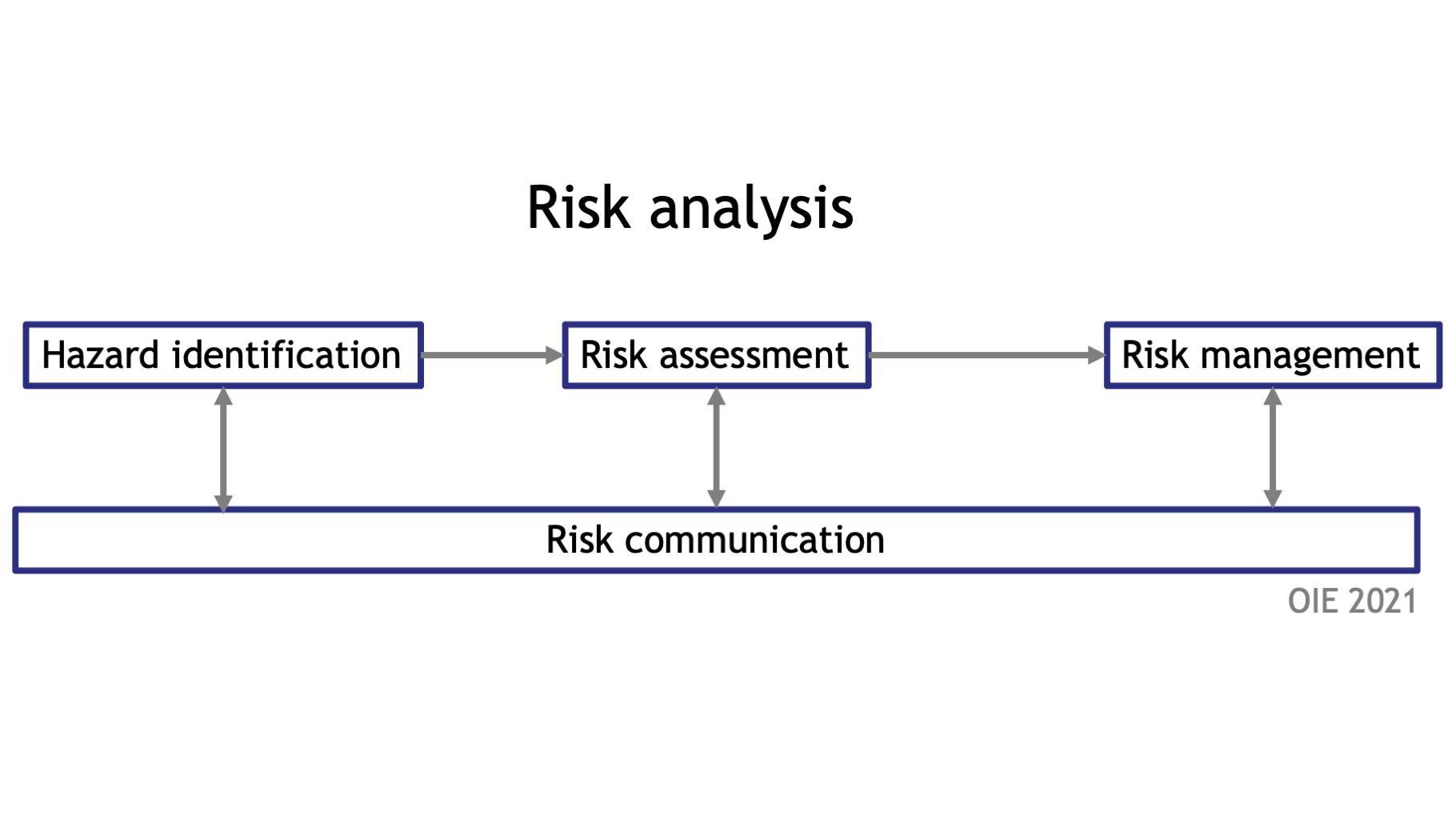
Risk assessment
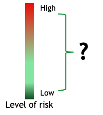
Triage
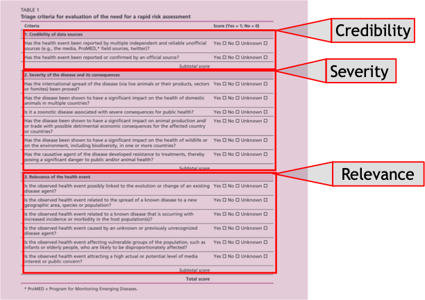
Triage
From this we could conclude:
- No need for further action
- More information needed
- Need for a RA
Formulating your question
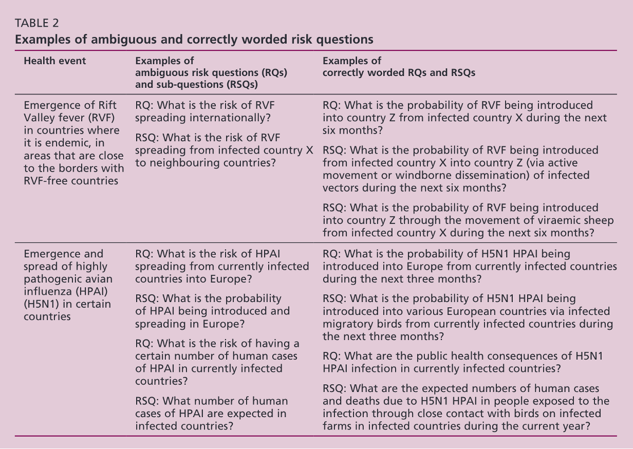
Formulating your question
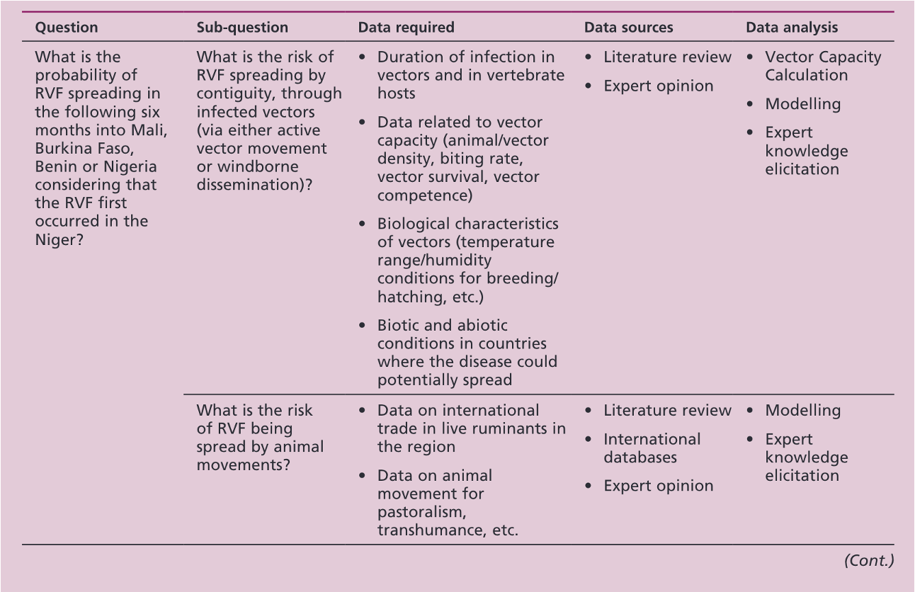
Data collection

To facilitate the search for data, eligibility criteria should be defined that take into account:
- Population of interest
- Variables of concern
- Possible geographical and time restrictions
Expert opinion

- Online questionnaire
- Expert panel
- Interviews
- Focus groups discussions
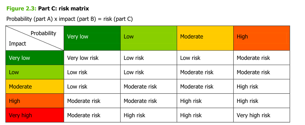
Performing the assessment
Type of outputs might include:
- Probability
- Probability of X event happening
- Probability of more than 10 introductions per year
- Consequences
- Number of animals/people infected
- Economic impact
Performing the assessment
Performing the assessment


Risk assessment in R
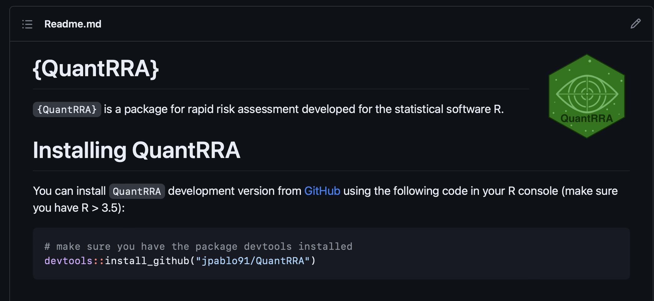
Risk assessment in R
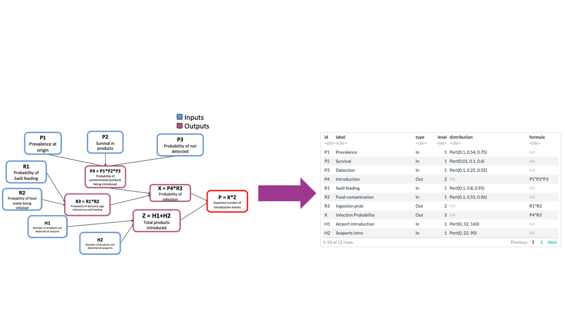
Risk assessment in R